by Norman Koren, Imatest LLC, April 30, 2024
The goal of this document is to compare the effects of demosaicing and sharpening (or bilateral filtering) on MTF measurements for the two most widely used test patterns — the slanted edge and the sinusoidal Siemens star. We are particularly interested in investigating the belief that Siemens stars (or sinusoidal patterns in general) are relatively unaffected by sharpening, so that their response approximates the original unsharpened system response.
Definitions
Sharpening — A process for making an image appear sharper by taking the original signal, then subtracting shifted, reduced-amplitude replicas (standard sharpening), or subtracting a reduced-amplitude, gaussian blurred version (unsharp masking or USM). These methods are uniform and (usually) linear, and are characterized by radius R and amount A. They have a transfer function with a peak at 0.25/R Cycles/Pixel = 0.25 C/P for the most common radius, R = 2. Described in detail in the Sharpening page.
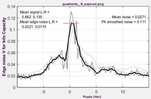
Bilateral filtering — a type of nonuniform and nonlinear filtering where regions of the image close to fine details or edges are sharpened (high frequencies are boosted), but regions away from edges are lowpass-filtered (smoothed; high frequencies are attenuated). The purpose is to reduce visible noise while maintaining a sharp appearance. Almost universal in JPEG files from consumer cameras. Can usually be detected by the presence of a strong peak in a plot the spatially dependent noise amplitude, ![]() (shown for images 3, 6, and 7). This plot is a part of the Image information metrics.
(shown for images 3, 6, and 7). This plot is a part of the Image information metrics.
Demosaicing — the process of transforming the signal from an image sensor (“mosaiced” with a color filter array, typically a (RGRG; GBGB…) Bayer array, into a three-channel RGB image. A key function of raw conversion, which also includes white balance, color correction, gamma-encoding, and often sharpening and noise reduction. Demosaicing is a type of interpolation that, in its simplest form (bilateral demosaicing), lowpass filters the signal (removes high frequency energy, mostly above 0.4 C/P). Sophisticated demosaicing algorithms use detected edges to try to recover this energy. Demosaicing quality is often better when performed by a raw conversion program, rather than in the camera.
Nyquist frequency — fNyq = 0.5 Cycles/Pixel, the highest frequency where the original signal can be reconstructed. Information above Nyquist is of interest because it indicates the likely presence of aliasing artifacts.
To explore the differences in performance between slanted edges and Siemens stars, we compare results from several images (simulated and from different cameras with different types of demosaicing). We found that sharpening behavior and response near and beyond the Nyquist frequency (fNyq = 0.5 C/P) are separate issues.
Image comparisons
1. Simulated image: no demosaicing
We applied a few tricks to obtain a fair comparison between the two patterns.
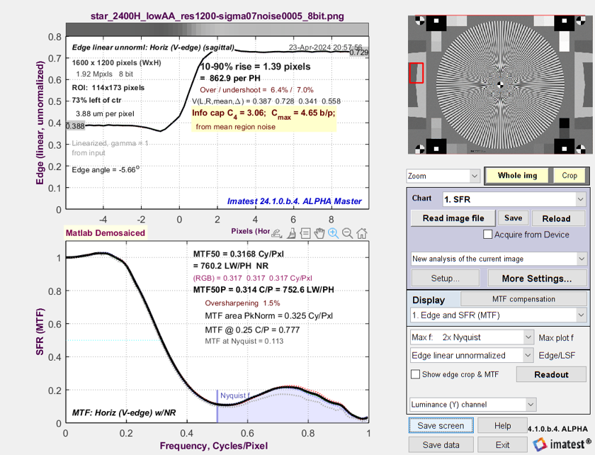
A 2400-pixel high image of a 50:1 contrast sinusoidal Siemens star (the ISO standard), which also contained 4:1 contrast slanted edges, was created with Imatest Test Charts. We adjusted the amount of anti-aliasing on the star to give results consistent with the edges.
To make the comparison fairer, we resized the 2400-pixel high images to 1200 pixels high using Irfanview, with the sharpen box checked. This was intended to remove differences due to the anti-aliasing routines for the star and edges, which are close but not identical. For comparison with real images, we added a small amount of gaussian blur (sigma = 0.7 pixels) and a tiny amount of gaussian noise (sigma = 0.0005 pixels).
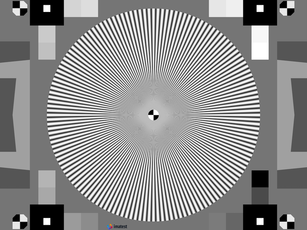
Simulated image with Siemens star and slanted edge, resized from 2400 to 1200 pixels high,
Blur sigma = 0.7 pixels; noise sigma 0.0005.
1. Simulated image: no demosaicing (continued)
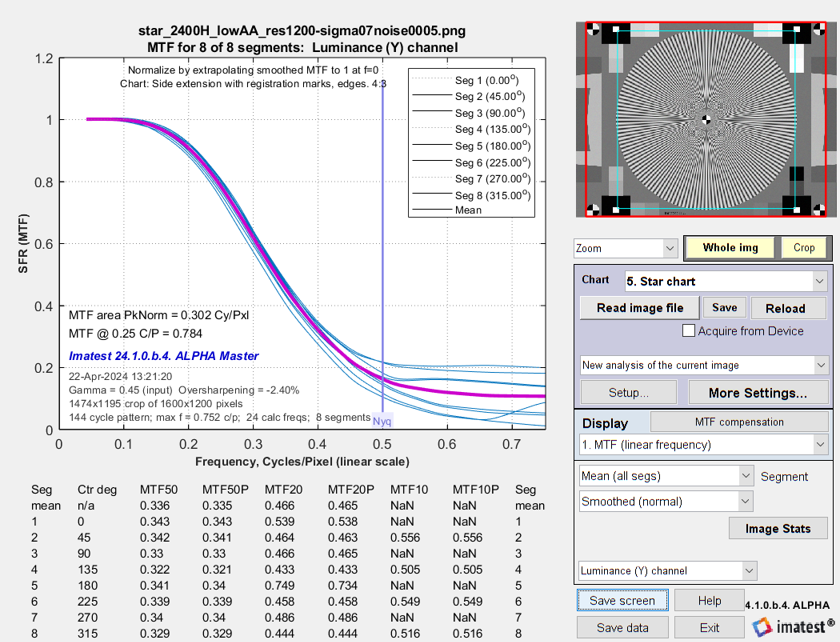
Results for simulated Siemens star. Mean MTF50 = 0.336.
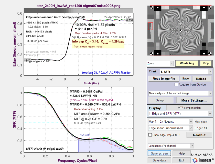 Results for simulated slanted edge (same image as star, above). MTF50 = 0.349.
Note the modest sharpening from the Irfanview resizing.
The results are close, but the average MTF is slightly lower for the star. (MTF50 = 0.336 for the star vs. 0.349 for the edge; around 0.17 at fNyq for the star vs. 0.23 for the edge). Note that the highest MTFs for the star (for specific angular regions) were very close to the edge.
All slanted-edge plots have a maximum display frequency of 1 C/P (2×fNyq), but the maximum for the star plot depends on the image size.
Both patterns have significant (though not identical) response above fNyq. It is possible that some of the response is an artifact of the resizing, but the important thing is that resizing affects the star and edge identically — hence makes the sine and edge response more consistent.
2. Simulated image: converted to 8-bit (monochrome) and demosaiced
The following two results are for the image in 1 (above), converted to monochrome (from 24 to 8 bit depth), then demosaiced using the MATLAB demosaicing routine.
(Note that the 8-bit undemosaiced images had MTF50 = 0.336 for the star and MTF50 = 0.3487 C/P for the slanted edge (both close).)
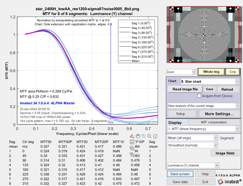
Results for simulated & demosaiced Siemens star
Results for simulated & demosaiced slanted edge (same image as star, above)
There were relatively small changes in the response. The star had lower response above fNyq than the edge.
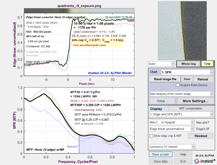
3. JPEG image from compact digital camera
Results for Siemens star from JPEG. No response above Nyquist.
Demosaicing and other raw-conversion functions were performed in the camera. (The demosaicing algorithm is different from image 2, above.)
Results for slanted edge from the same JPEG.
Right: noise amplitude, \(\sqrt{N(x)}\).
The plot below shows the spatially dependent noise amplitude, \(\sqrt{N(x)}\). As we discuss above and in the documentation for Image information metrics, a strong peak indicates the presence of bilateral filtering.
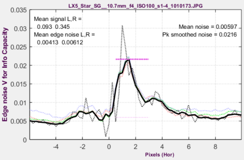
The Siemens star and slanted edge appear to be sharpened by similar amounts (just a slightly larger MTF peak for the edge) with radius ≈ 2 in both cases, even though the noise amplitude plot on the right clearly indicates bilateral filtering—which could reduce sharpening for the Siemens star.
The big difference in the two results is that the star has nearly zero response above Nyquist (fNyq = 0.5 C/P), while the edge has very significant response (0.4 at fNyq). The low response for the star and the high response for the edge is most likely due to interpolation in the camera’s fast but low-quality demosaicing, though it might be related to bilateral filtering, which is definitely present.
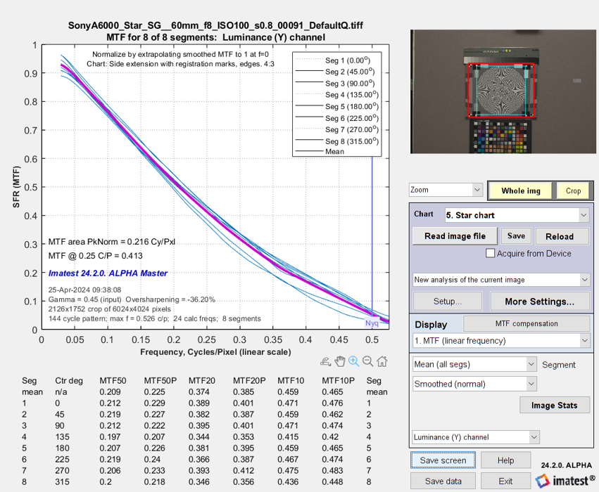
4. LibRaw-converted (unsharpened) image from compact digital camera
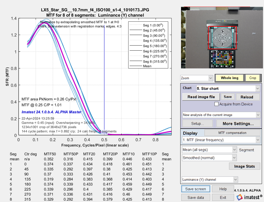
Results for Siemens star from the LibRaw-converted image (unsharpened)
The same image as the JPEG in 3 was converted with LibRaw. This is the unsharpened result.
Information capacity = 3.4 bits/pixel.
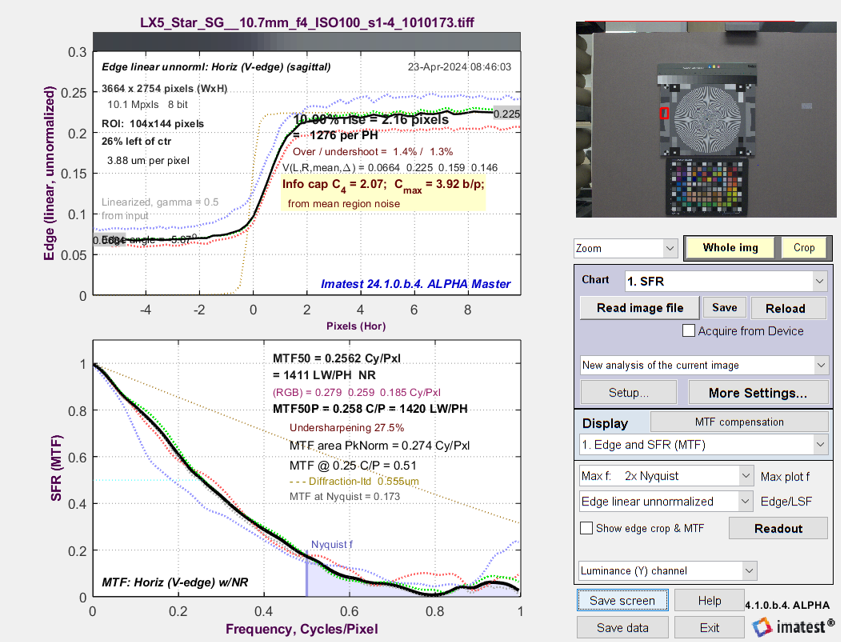
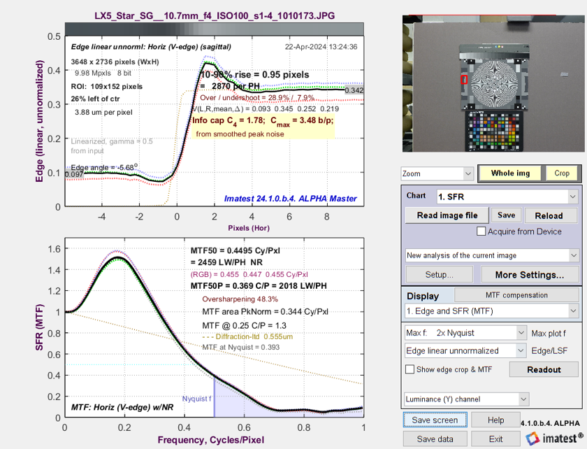
Results for slanted edge from the LibRaw-converted image (unsharpened)
Results are similar, but MTF50 for the edge (0.256 C/P) is somewhat larger than for the star (0.227) MTF at Nyquist is approximately 0.18 for the edge vs. 0.07 for the star. Unlike the camera JPEG, there is some response above Nyquist for the star, but it is lower than for the edge.
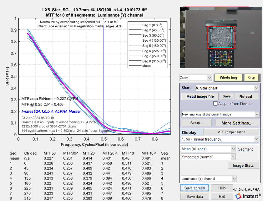
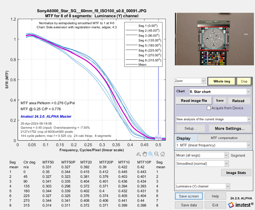
5. LibRaw-converted & sharpened image from compact digital camera
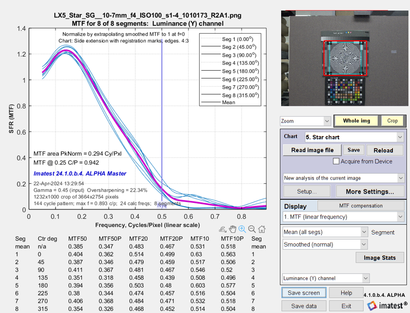
Results for Siemens star from the sharpened LibRaw-converted image
The same image as the JPEG in 3 was saved as raw and converted with LibRaw. A modest amount of sharpening (R2A1; Radius = 2, Amount = 1) was applied to make it easier to compare with the JPEG results. (Saturation was an issue with more sharpening.)
Information capacity = 3.36 bits/pixel. Unchanged from the unsharpened image. 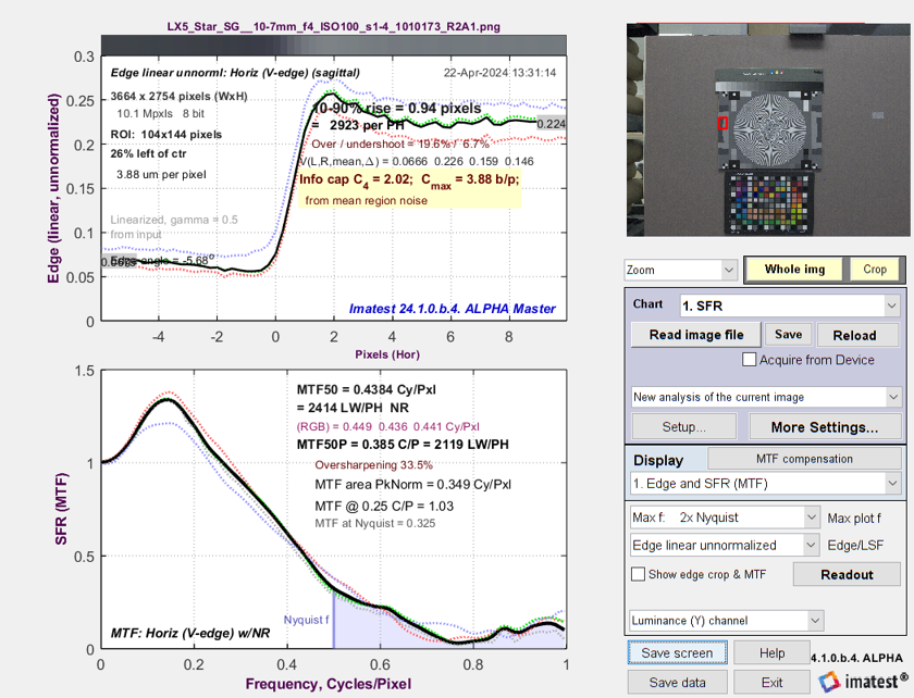
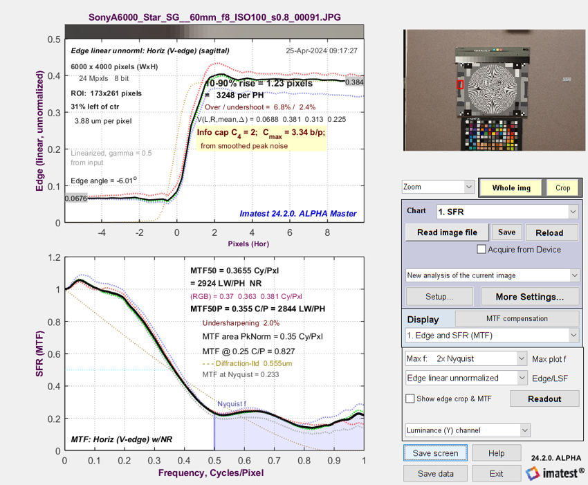
Results for slanted edge from the sharpened LibRaw-converted image.
The key thing to note is that sharpening affects both star and edge MTF, but the edge is just slightly more strongly sharpened. Unlike the JPEG, the star has some response above Nyquist. Information capacity for both patterns is unaffected by sharpening. (It is slightly lower for the star than Cmax for the edge.)
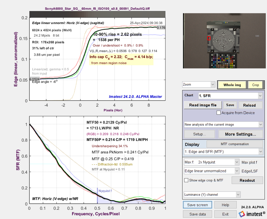
6. JPEG image from 24-megapixel Micro Four-Thirds digital camera
Because this camera is from a different manufacturer from 3, we expect the in-camera demosaicing routine to behave differently.
Results for Siemens star from JPEG. As with 3, there is no response above Nyquist.
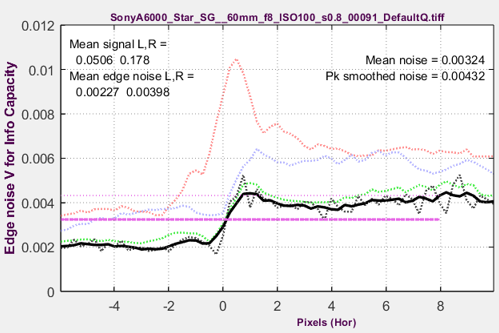
Results for slanted edge from the same JPEG. Right: noise amplitude (\(\sqrt{N(x)}\)).
The artifacts above fNyq are particularly severe.
Both response curves show a bump from moderate amounts of sharpening. Bilateral filtering, which is common in JPEGs from cameras, does not appear to be strong.
7. LibRaw-converted (unsharpened) image from 24-megapixel digital camera
The same image as the JPEG was converted with LibRaw. This is the unsharpened result.
Results for Siemens star from the LibRaw-converted image (unsharpened)
Results for slanted edge from the LibRaw-converted image (unsharpened)
Noise amplitude (\(\sqrt{N(x)}\)) has no peak (indicating no bilateral filtering).
Results are similar. The MTF50 for the edge (0.213 C/P) is nearly identical to for the star (0.209). However, MTF at fNyq is double for the edge (0.11 vs. 0.05) — a ratio similar to Figure 4.
Verification of the slanted-edge calculation
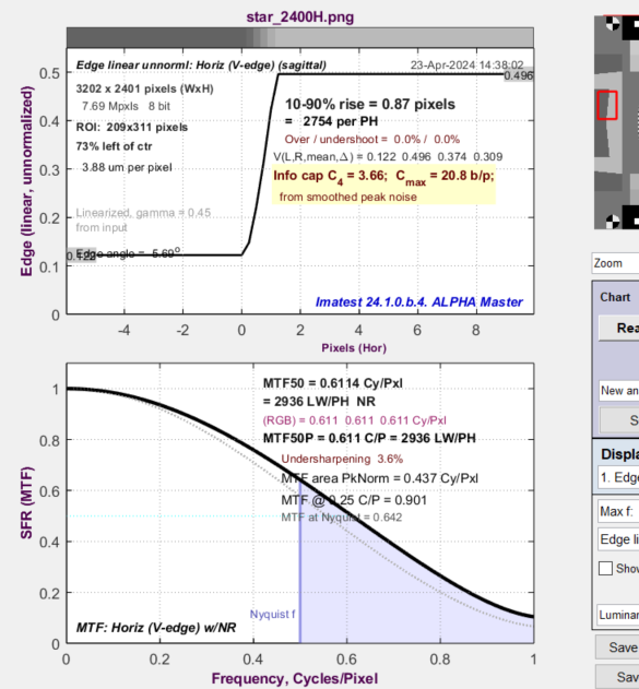 There are two places on the Imatest website where the slanted-edge calculation is verified.
LSF correction factor for slanted-edge MTF measurements verification. This is for an idealized edge that changes from light to dark linearly over a distance of one pixel. Here is the result for the slanted-edges in the latest Siemens star (with edge) Test Charts pattern.
The equations for the MTF are on the above link. The expected value is MTF(fNyq) = 0.6366, which is very close to the result shown on the right (0.642).
Validating the Imatest slanted-edge calculation compares a somewhat blurred sine pattern and edge. Slanted-edges are compared with sine patterns, but the edge rise distance on this page is not exactly one pixel, so results are somewhat different from the previous link.
Summary
In preparing this document we realized that two separate issues affect the comparison of slanted edges with Siemens stars.
- Sensitivity to sharpening — Depending on how you classify them, there are two or three types of sharpening, all characterized by radius R and amount A, where the peak sharpening transfer function is at 0.5/R (0.25 C/P for the most common sharpening radius, R = 2).
- Uniform sharpening, which can either be standard or USM (unsharp mask),
- Bilateral filtering (described in documentation for Image information metrics), where areas near sharp edges are sharpened, but smooth areas (away from edges) may be smoothed (lowpass-filtered or blurred). Bilateral filters are nearly universal in JPEG images from consumer cameras. The amount of lowpass filtering, sharpening, and the transition threshold varies for different cameras.
- Response near and above Nyquist (f > 0.4×fNyq, where fNyq = 0.5 C/P) — affected by the demosaicing algorithm, which can be different when performed in the camera or in a separate program on a computer (not in the camera; Imatest uses LibRaw).
- In-camera demosaicing (used to produce JPEGs) are optimized for maximum speed and minimum power consumption. Quality may be compromised.
- Demosaicing programs run on computers are primarily optimized for quality; speed is less critical.
- In-camera demosaicing (used to produce JPEGs) are optimized for maximum speed and minimum power consumption. Quality may be compromised.
Image summary
|
# |
Source |
Processing |
|
1 |
Simulated (Test Charts) |
Resize 2400H → 1200H, blur σ = 0.7, noise σ = 0.0005 |
|
2 |
#1 |
Convert to 8-bit monochrome, MATLAB demosaicing |
|
3 |
Compact camera (Lumix LX5) |
JPEG (sharpened) |
|
4 |
Compact camera (Lumix LX5) |
Raw, LibRaw demosaicing |
|
5 |
Compact camera (Lumix LX5) |
Raw, LibRaw, USM sharpened R2A1 to compare with #3 |
|
6 |
Micro 4/3 camera (Sony A6000) |
JPEG (sharpened) |
|
7 |
Micro 4/3 camera (Sony A6000) |
Raw, LibRaw demosaicing |
Results — Sensitivity to sharpening
Images 3, 5, and 6 are sharpened. 3 and 6 are sharpened in different cameras. 5 was demosaiced with LibRaw and uniformly sharpened (uniformly) using Unsharp Mask with R2A1; Radius = 2, Amount = 1.
The in-camera JPEG from compact digital cameras 3 and 6 show similar sharpening for the edge and star (slightly more for the edge). Because JPEGs from most cameras have bilateral filtering (nonuniform sharpening) we expected to see a larger difference. The dramatic difference at fNyq, where there is strong response for the edge, but essentially zero response for the star, is a separate issue related to demosaicing, described below.
Results — Response near and above Nyquist (fNyq = 0.5 C/P)
Response near and above Nyquist is strongly affected by demosaicing, which can vary significantly between cameras and external raw converters.
Demosaicing — in its simplest form is an interpolation process, which acts as a lowpass filter. High quality demosaicing is aware of detail in the individual channels (especially edges) and adjusts the interpolation to maintain detail.
Results — The response of the simulated, undemosaiced image 1 is relatively close for the star and edge, with the edge having slightly larger response at fNyq (0.23 vs. 0.17). This is our baseline (results with no image processing).
When image 1 is interpreted as Bayer raw and demosaiced using the high-quality MATLAB demosaicing routine (image 2), the changes are relatively small. MTF at fNyq is slightly lower for both cases, but the comparison is unchanged.
Images 4, 5, and 7, stored in raw format then demosaiced by LibRaw (high quality), have responses comparable to images 1 and 2, but the MTF at Nyquist is higher for the slanted edges relative to the stars — around double.
Images 3 and 6, JPEGs converted in the cameras, have major differences between edges and stars at f > 0.4 C/P. There is essentially no response above Nyquist for the stars. But for edges, MTF above Nyquist is much larger than for LibRaw-converted images. This response appears to be mostly artifacts resulting from low-quality in-camera demosaicing.
For in-camera raw conversion,MTF for f ≥ fNyq is often boosted (with artifacts) for slanted edges, but severely attenuated (effectively removed) for Siemens stars. Neither shows the whole picture.
Images 3 and 6 are examples of low quality demosaicing — common in camera JPEGs. Edge MTF is aggressively maintained, but artifacts are created in the process. MTF for the stars is strongly attenuated for f ≥ fNyq. [Note: this is unrelated to JPEG compression.] By comparison, LibRaw-converted images 4, 5, and 7 maintain edge response with smaller artifacts and maintain some star response above Nyquist (absent in the camera JPEGs).
So which pattern is better?
Tricky question. Both are good, and they produce different results because demosaicing algorithms respond differently to the different patterns.
But as founder of Imatest and author of this document, I (NLK) offer an opinion. I prefer slanted edge measurements for several reasons.
- Our perception of sharpness is largely based on edges, not on sinusoidal patterns.
- Demosaicing routines (especially off-camera) recover more of the sharpness lost to interpolation for edges than for sinusoidal features (such as the Siemens star). Separate raw converter programs perform better. In-camera demosaicing is usually inferior, often creating artifacts in slanted edges at f ≥ fNyq while severely attenuating high frequency response for sinusoidal patterns. With in-camera demosaicing, neither pattern produces results for f near and above fNyq sufficient to characterize the camera. Both results are needed for a fuller picture.
- Slanted-edge analysis has several other well-known advantages. Edges are generally smaller, making it practical to map sharpness over the surface of the image. Computations are faster. And for 4:1 contrast edges (specified by ISO 12233), saturation is rarely a problem, except when the image is overexposed or sharpening is excessive. And when sharpening is excessive, large spikes (“halos”) near edges represent the actual performance of the camera quite well.
- Low resolution images (common in medical endoscopes) may have insufficient resolution with Siemens stars to allow space for a low frequency reference, which is critical for calculating MTF. (This can be mitigated by reducing the number of cycles in the star.) Light falloff (vignetting) can also adversely affect the low frequency reference. With slanted edges, a low frequency reference is taken for granted because it is easy to obtain.
- Image information metrics (measurements related to information capacity, including object and edge detection performance) are calculated using MTF for f < fNyq (avoiding frequencies where the results for the two patterns strongly diverge). These metrics are currently available for slanted edges. With some effort, they could be added to Siemens star results at customer request.
- The star response represents a wider range of angles than edges, but we have rarely observed new information of interest over a range of angles. All the star plots above contain results for 8 angular regions, and results for the regions are very close. Of course, it is possible that something surprising might show up in the star that would be missed with the edge.·
- A customer had an extremely oversharpened image (huge spatial and frequency domain overshoots), and was unhappy because slanted-edge MTF never dropped to the 20% level, and hence MTF20 could not be measured. In this case we need to educate the customer that:
- Edge-MTF20 is not a good system performance metric for severely oversharpened images. Even Edge-MTF50 has its problems, and may not represent system performance, as described in the 2020 paper, Correcting Misleading Image Quality Measurements.
- Extreme oversharpening degrades system performance, as quantified by object and edge detection metrics SNRi and Edge SNRi, described in Image Information metrics.
- Because JPEGs from cameras may have severely attenuated Siemens star response at and above fNyq (the result of interpolation in low-quality demosaicing; see images 3 and 6), MTF20 and MTF10 can almost always be measured from stars. But the measured result is dominated by the lowpass filtering of the demosaicing, and hence does not represent system performance.
Conclusions
Both patterns produce similar results below the Nyquist frequency, fNyq = 0.5 C/P.
The slanted edge is preferred at Imatest because it is more convenient: It is smaller, faster, and better for mapping MTF over the image surface. The full set of image information metrics is available.
Star and edge results can diverge around fNyq for images demosaiced in cameras because cameras tend to have lower quality demosaicing than separate raw converters (LibRaw, etc.), resulting in artifacts in edge response and nulls in star response near and above fNyq. And JPEG images from cameras also usually have bilateral filtering.
Raw (sensor) response cannot be reliably recovered from JPEG images captured in cameras. However, much useful information (including a reasonable estimate of information capacity) can still be obtained.
Miscellaneous notes
Linear systems and their limits
Imaging systems are mostly linear (or can be linearized by inverting the gamma encoding of digital numbers). Linear operations have simple, predictable behavior: For a linear operation H on xn(t) such that \(y_n (t)=H(x_n (t))\), then \(αy_1 (t)+βy_2 (t)=H(x_1 (t)+βx_2 (t))\) [from Wikipedia]. Standard sharpening and lowpass filtering are linear operations. Unsharp Masking (USM), as commonly defined, is linear, though the MATLAB implementation is not.
Imaging systems, like all linear systems, have limits, and things get interesting when the limits are reached. If imaging systems were perfectly linear, slanted edges and Siemens stars would have identical response. Imaging systems are affected by several types of nonlinearity.
- Stray light, also called veiling glare or flare light, affects measurements when strong light sources (such as the sun) fog the image. In addition to simple measurements, Imatest offers sophisticated hardware for measuring stray light.
- Saturation, which occurs then the limits of allowable digital numbers are reached, can cause serious errors in MTF measurements. Saturation can occur when images are under or overexposed, chart contrast is too high, or sharpening is excessive. Described below.
- Bilateral filtering, described in the documentation for Image information metrics), in which regions of the image close to edges are sharpened (high frequencies are boosted), but regions far from edges are lowpass-filtered (high frequencies are attenuated). Bilateral filtering is nonuniform as well as nonlinear. Almost universal in JPEG files from consumer cameras.
- Demosaicing (the primary cause of differences between slanted-edge and Siemens star response) is a type of interpolation that lowpass filters much of the image, but behaves differently near edges. Discussed below.
The frequency response of interpolation (which includes demosaicing)
We learned how interpolation affects MTF response when we were struggling with an inconsistency in the image information metrics: Noise Equivalent Quanta (NEQ) was unexpectedly changing when the image was sharpened. The story is chronicled on Interpolated slanted-edge SFR (MTF) calculation.
We observed that slanted-edge MTF often had high frequency artifacts that were absent in the Siemens star MTF. We thought these might be the cause of the NEQ inconsistency. To remedy the issue, we applied interpolation to the slanted-edge binning calculation. This made MTF from slanted edged nearly identical to Siemens stars — the high frequency artifacts were eliminated.
But interpolated binning failed to fix the NEQ inconsistency (we eventually found another cause). We realized that interpolation caused the signal to be lowpass-filtered with a sinc2(fT) transfer function for sampling interval T. This cleaned up the high frequency artifacts in the slanted-edge MTF, but also filtered the Siemens star response, which wasn’t obvious because the star had no high frequency artifacts to begin with.
Demosaicing is also a form of interpolation, but with nonuniform processing. It behaves differently in the vicinity of edges, restoring MTF response that would otherwise be filtered out. This accounts for the difference in slanted-edge and Siemens star MTF response, which is usually much greater for demosaicing in cameras. High quality raw conversion algorithms, such as LibRaw or MATLAB Demosaic, used in Imatest, reduce the discrepancy between MTF results for the two patterns (images 2, 4, 5, and 7).
Saturation and MTF
When an image saturates (or clips), a sharp corner can form at the boundary of the clipped region that causes the MTF measurement to erroneously increase. Normally saturation happens at the limits of the digital number range defined by the bit depth, for example, 0-255 for bit depth = 8 or 0-65535 for bit depth = 16.
But we sometimes see clipping at other levels, sometimes caused by strange (possibly bad) image processing in prototype cameras, and occasionally in images with specialized color spaces, for example, Rec. 709 only allows digital numbers between 16 and 235 for bit depth = 8. Rec. 2020 also has limits.
It is important to watch for unexpected saturation, which can adversely affect results. Saturation may be less than obvious when just one of the three color channels saturates. Exposure may need to be adjusted to minimize saturation.
Low quality cameras
The cameras used in this document were all good quality. I was recently shown images from a cheap camera that appeared to strongly compress the image. (Compression can sometimes be identified by blocking artifacts).
Here is an enlarged portion of a slanted-edge pattern for such a bad image. All sorts of ugly, nasty artifacts are visible.
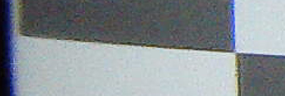
 This image had a high slanted-edge MTF at Nyquist (lower plot on the right), but it had zero sinusoidal response near Nyquist, either due to low-quality demosaicing or bilateral filtering, which appeared to be extremely strong, as indicated by the figure below.
While demosaicing is the most likely cause of the discrepancy, bilateral filtering could be involved. Their effects can be confused in “black box” cameras.
 In cases like this, neither slanted edge nor Siemens star results by themselves can completely characterize the camera. Both results are required. And charts like Log Frequency-Contrast add more to the picture.
Simply put the slanted-edge and sinusoidal star response indicate the camera’s response to two different types of input.
Results for Additional Cameras
Samsung Galaxy S4
Log F-Contrast results are of great interest because they show the effects of contrast on sinusoidal MTF measurements. In most cases, the results for the top (high contrast) row corresponds to Star chart measurements.
 Samsung Galaxy S4, MTF curves for Log F-Contrast, Samsung Galaxy S4, MTF curves for Log F-Contrast,rows 1-19 in steps of 3, camera JPEG @ ISO 125 |
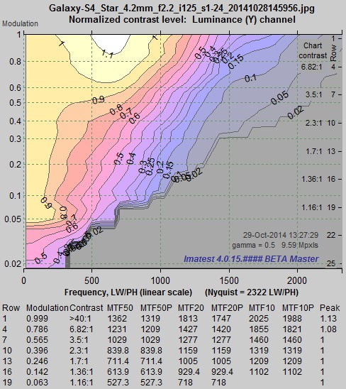 Samsung Galaxy S4, MTF contours for Log F-Contrast, Samsung Galaxy S4, MTF contours for Log F-Contrast,camera JPEG @ ISO 125 |
The Galaxy S4 has excellent response with moderate sharpening at high contrast, but sharpening decreases and noise reduction increases rapidly as contrast drops. This is common behavior in small-sensor camera phones. We expect texture detail to be weak.
|
Siemens Star measurements The MTF response of the Siemens Star displays moderately strong sharpening: nearly identical to row 1 of the Log F-Contrast chart, shown above.
|
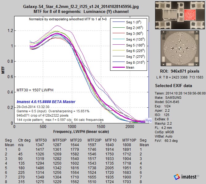 Samsung Galaxy S4, MTF for Siemens Star, Samsung Galaxy S4, MTF for Siemens Star,camera JPEG @ ISO 125 |
|
Slanted-edge measurements Autofocus is temperamental with the Galaxy S4, and it appears that the image used for the Log F-Contrast, Siemens Star and ~12:1 and 2:1 edges was not focused as well as the SFRplus image used for the 4:1 edges. For simplicity we show only the Edge/MTF plot for 4:1 contrast (the SFRplus chart), and we summarize the other results in a table.
*from SFRplus image, which appears to be in better focus. MTF for the 4:1 slanted-edge is nearly identical to MTF for the Siemens star (as well as the top row of the Log F-Contrast image). |
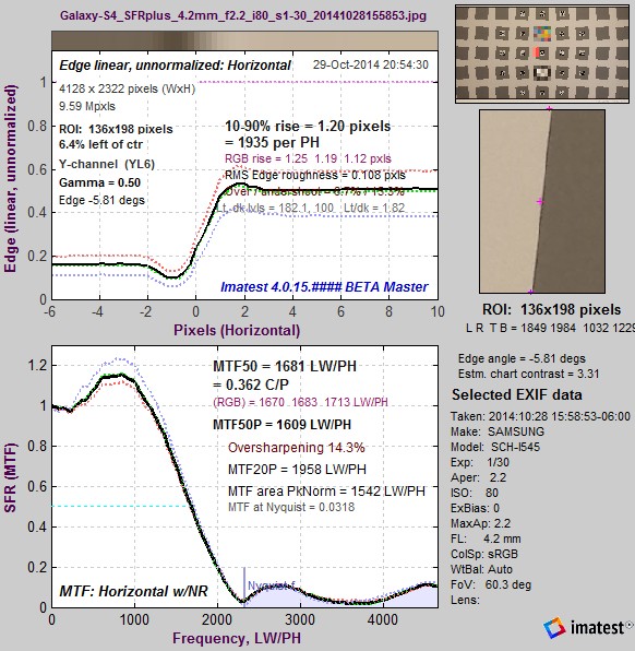 Samsung Galaxy S4, MTF for 4:1 slanted-edge, Samsung Galaxy S4, MTF for 4:1 slanted-edge,camera JPEG @ ISO 80 |
Summary— For the Samsung Galaxy S4 phone, the Siemens Star MTF is very similar to the 4:1 contrast Slanted-edge (and between the 2:1 and ~12:1 edges on the same chart as the star).
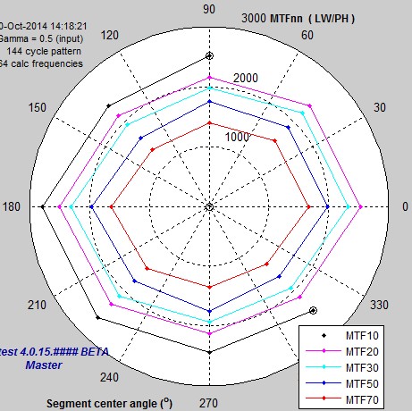
Panasonic Lumix DMC-G3
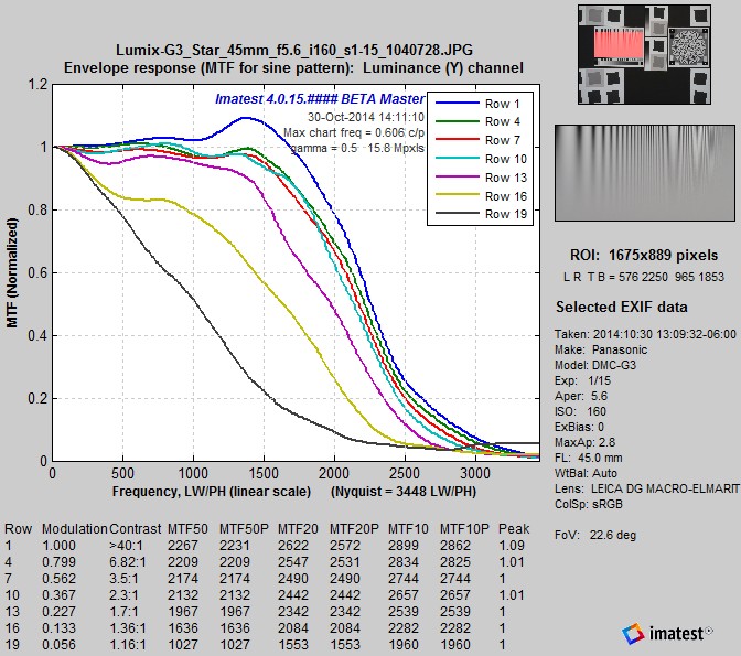 Lumix DMC-G3, MTF curves for Log F-Contrast, Lumix DMC-G3, MTF curves for Log F-Contrast,rows 1-19 in steps of 3, camera JPEG @ ISO 160 |
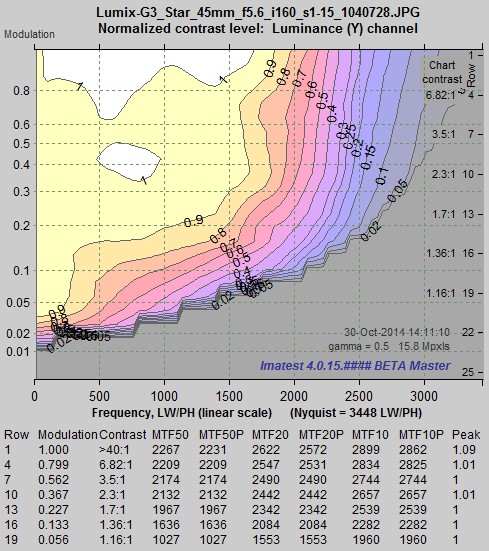 Lumix DMC-G3, MTF contours for Log F-Contrast, Lumix DMC-G3, MTF contours for Log F-Contrast,camera JPEG @ ISO 160 |
The DMC-G3 behaves very differently from the Galaxy S4. It has a moderate sharpening peak and it maintains contrast quite well down to modulation around 0.2 (about 1.6:1 contrast), after which it falls rapidly. Results are very close to results we’ve analyzed from Imaging-Resource.
|
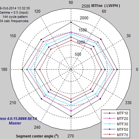
Siemens Star measurements
The MTFnn contour plot is also a little different from the Samsung Galaxy G4: diagonal MTFs are slightly closer to the Horizontal and Vertical MTFs. |
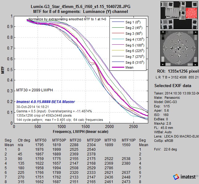 Lumix DMC-G3, MTF for Siemens Star, Lumix DMC-G3, MTF for Siemens Star,camera JPEG @ ISO 160 |
|
Slanted-edge measurements For simplicity we show only the Edge/MTF plot for 4:1 contrast (the SFRplus chart), and we summarize the other results in a table.
|
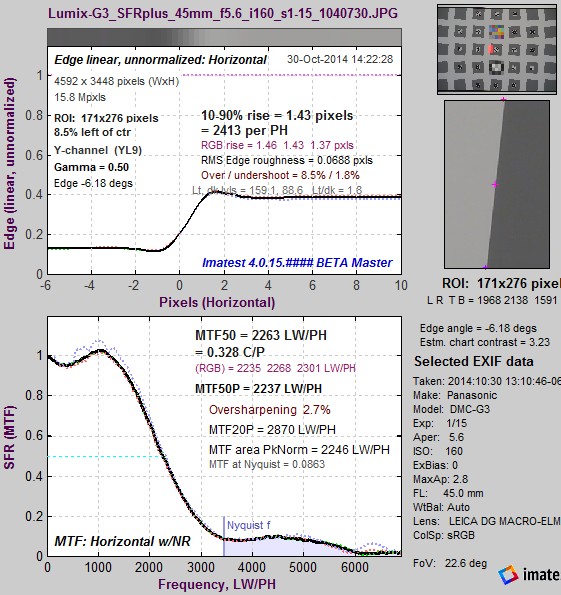 Lumix DMC-G3, MTF for 4:1 slanted-edge, Lumix DMC-G3, MTF for 4:1 slanted-edge,camera JPEG @ ISO 160 |
Summary— For the Panasonic Lumix DMC-G3, the Siemens Star MTF is very similar to the 4:1 contrast Slanted-edge (and between the 2:1 and ~12:1 edges on the same chart). But it is unusual in that it’s lower than the top row of the Log F-Contrast chart.
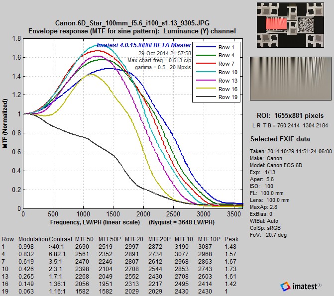
Canon EOS-6D
 Canon EOS-6D, MTF curves for Log F-Contrast, Canon EOS-6D, MTF curves for Log F-Contrast,rows 1-19 in steps of 3, camera JPEG @ ISO 100 |
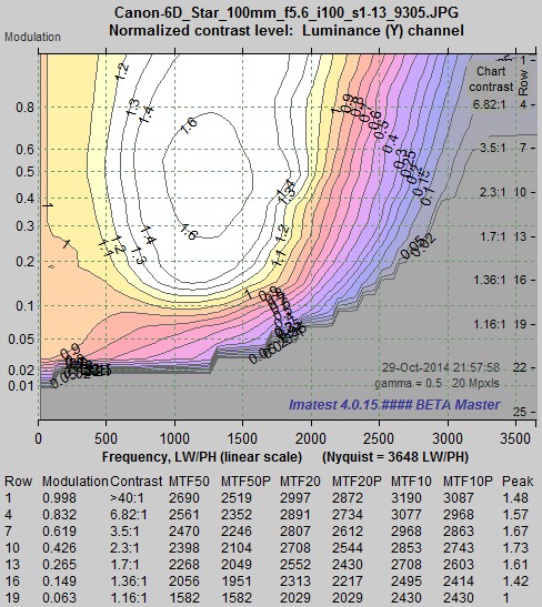 Canon EOS-6D, MTF contours for Log F-Contrast, Canon EOS-6D, MTF contours for Log F-Contrast,camera JPEG @ ISO 100 |
The EOS-6D has a very strong sharpening peak. MTF drops slowly between maximum modulation and modulation around 0.15 (about 1.5:1 contrast). It drops quite rapidly below modulation = 0.15. It is interesting to compare these results with results we’ve analyzed from Imaging-Resource. The general features of the contours are similar, but their sharpening was much weaker at high modulation levels (near the top of the chart). The reason seems to be that their image is lighter, hence there is less “headroom” for sharpening boost without running into saturation. Canon may well reduce sharpening in light, high-contrast regions to minimize saturation effects. (We haven’t done systematic tests of how exposure affects MTF response.)
|
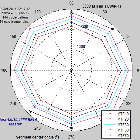
Siemens Star measurements The MTF response of the Siemens Star displays moderately strong sharpening,but it’s different from most of the cameras we tested in that it’s significantly lower than row 1 of the Log F-Contrast chart.
|
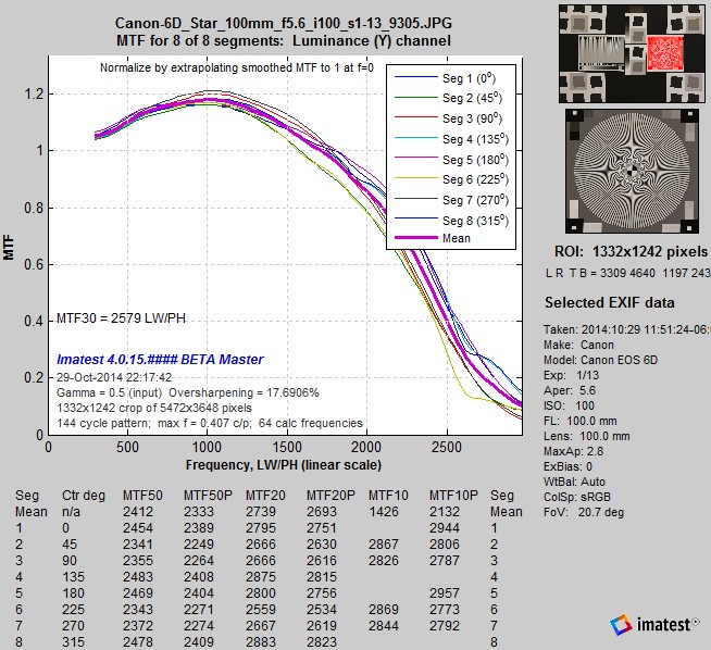 Canon EOS-6D, MTF for Siemens Star, Canon EOS-6D, MTF for Siemens Star,camera JPEG @ ISO 100 |
|
Slanted-edge measurements To keep things simple, we show only the Edge/MTF plot for 4:1 contrast (the SFRplus chart), and we summarize the other results in a table.
|
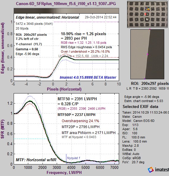 Canon EOS-6D, MTF for 4:1 slanted-edge, Canon EOS-6D, MTF for 4:1 slanted-edge,camera JPEG @ ISO 100 |
Summary— For the Canon EOS-6D, the MTF curves for the Siemens Star and the 4:1 contrast Slanted-edge is very similar. But it is unusual in that it’s lower than the top row of the Log F-Contrast chart. There is some complex image processing happening here.
Nikon D800E
Because of the extremely high resolution of the D800E (36 megapixels; no anti-aliasing filter) we had to move the camera further than usual from the charts. When framed the same as the other cameras we couldn’t get to high enough spatial frequencies on the Siemens star.
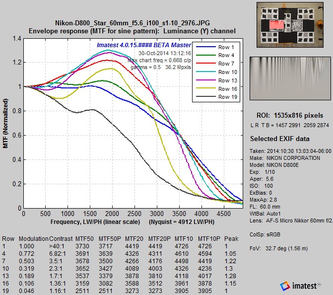 Nikon D800E, MTF curves for Log F-Contrast, Nikon D800E, MTF curves for Log F-Contrast,rows 1-19 in steps of 3, camera JPEG @ ISO 100 |
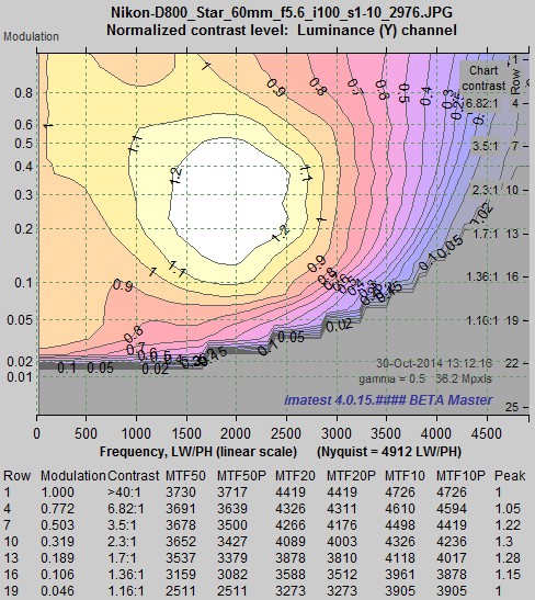 Nikon D800E, MTF contours for Log F-Contrast, Nikon D800E, MTF contours for Log F-Contrast,camera JPEG @ ISO 100 |
The Nikon D800E’s high frequency response is considerably more extended than the Canon EOS-6D, which is what you would expect of a 36 megapixel sensor without an Anti-Aliasing filters (vs. 20 megapixels with an AA filter). It is interesting to compare these results with results we’ve analyzed for the D800 (which has an AA filter) from Imaging-Resource. The general features of the contours are similar, but the response of the D800E is about 20% more extended.
|
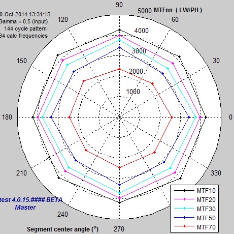
Siemens Star measurements The MTF response of the Siemens Star displays moderate sharpening: similar to row 1 of the Log F-Contrast chart, shown above.
|
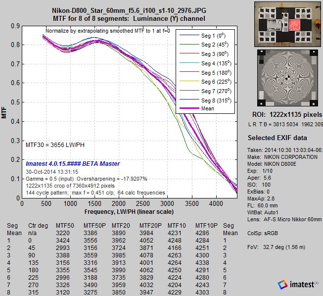 Nikon D800E, MTF for Siemens Star, Nikon D800E, MTF for Siemens Star,camera JPEG @ ISO 100 |
|
Slanted-edge measurements The relationship between sharpness and contrast is quite different for the D800E than for most other cameras. This is because noise reduction is not significant until contrast falls below 1.7:1. (The 0.5 (MTF50) contrast line in the Log F-Contrast contour plot, above, is nearly vertical.)
|
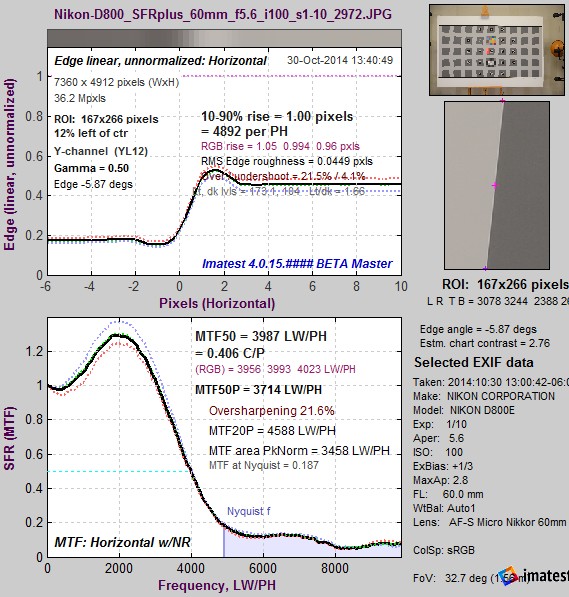 Nikon D800E, MTF for 4:1 slanted-edge, Nikon D800E, MTF for 4:1 slanted-edge,camera JPEG @ ISO 100 |
|
For the D800E, the sharpening peak increases as contrast decreases, reaching a peak at modulation = 0.3, equivalent to 2.3:1 contrast. The primary reason seems to be that the highlights are compressed due to the “shoulder” in the response curve: the region where the slope decreases, shown in the tonal response curve, below.
There is also an unusual shift in the lower pixel level for the high contrast curve at high spatial frequencies (also visible on the D800 image from Imaging-Resource). Along with the compression, this explains the reduced MTF for the high contrast region of the Log F-Contrast image and the Siemens Star chart. |
Pixels (used to calculate MTF) for Row 1 (highest contrast) and 10 (2.3:1 contrast, where MTF is highest). |

Summary— The Nikon D800E is rather unusual in that its sinusoidal MTF response is highest (due to maximum sharpening) around contrast = 2.5:1 and drops at the highest levels. This may be done intentionally in the signal processing pipeline to minimize saturation effects. As a result of this processing, the (>50:1 contrast) Siemens Star MTF is distinctly lower than the (4:1 contrast) slanted-edge. This does not mean that the Siemens Star is less sensitive to software sharpening.