Stray light (flare) documentation pages
Introduction: Intro to stray light testing and normalized stray light | Outputs from Imatest stray light analysis | History
Background: Examples of stray light | Root Causes | Test overview | Test factors | Test Considerations | Glossary
Calculations: Metric image calculations | Normalization methods | Light source mask methods
Instructions: High-level Imatest analysis instructions (Master and IT) | Computing normalized stray light with Imatest | Motorized Gimbal instructions
Settings: Settings list and INI keys/values | Configuration file input
Page Contents
This page provides a description of Imatest’s Normalization Methods.
Normalization “factors out” the level of the light source used in testing. It allows for easier comparison between tests performed with different hardware.
Normalization Methods
The Imatest stray light source analysis has several options or methods available for normalizing the images under test.
None
Description
With the None normalization method, the test images are not normalized.
This is the simplest of the normalization methods (don’t normalize). It has two main benefits:
-
- Easy to get started (no extra info is needed).
- Stray light metric will be in units of digital number (DN) and similar intuition to noise levels can be used.
- Can directly analyze and see how the stray light manifests itself in the images after any image signal processing.
Inputs
-
- None
Normalization Factor
The normalization factor for this method is always 1.
Metric Range
| Calculation | Best Possible Measurement | Worst Possible Measurement |
| Transmission | 0 | Maximum digital number in an image |
| Attenuation | +∞ | One divided by the maximum digital number in an image |
Level
Description
With the Level normalization method, the user enters the level in units of digital number that is used to normalize the images under test. A normalization level can be computed using the methods described in the Normalization Compensation section. An example level calculation is provided here.
Inputs
-
- Normalization Level in digital numbers [DN]
Normalization Factor
The normalization factor for this method is the normalization level entered by the user.
Metric Range
| Calculation | Best Possible Measurement | Worst Possible Measurement |
| Transmission | 0 | 1 |
| Attenuation | +∞ | 1 |
Note: the above levels assume that the user-provided level will produce stray light in a 0-1 range for a transmission calculation. It is possible to choose a level that breaks this assumption.
Reference Image
Description
With the Reference Image normalization method, a reference image is used for computing the point source rejection ratio (PSRR) metric or extended source rejection ratio (ESRR) [1]. The level from the direct image of the source within the reference image is used to normalize the images under test. This image may require a lower light level (e.g., with the use of ND filters) and/or shorter camera exposure time than that which was used for the test images, so that the direct image of the source is not saturated in the image. The normalization can be compensated to produce a “test image-equivalent” normalization factor by using the normalization compensation settings (ND filter settings and ratio settings).
See the Normalization Compensation section for background information about the reference image and compensation settings.
Inputs
-
- Reference image filename (fully qualified path to image file)
- Aggregation method: how to aggregate the “direct image pixels” into a single number
- Reference image compensation factors: Used to compensate the base normalization factor derived from the reference image
- ND measurement type (none, density, or transmission)
- ND measurement value (density or transmission value of the ND filter, if used for the reference image)
- Integration time ratio: The ratio of the reference integration time to the analysis integration time (i.e., the value for the reference image divided by the value for the analysis image)
- Gain ratio: The ratio of the reference gain to the analysis gain (i.e., the value for the reference image divided by the value for the analysis image)
- Light level ratio: The ratio of the reference light level to the analysis light level (i.e., value for reference image divided by the value for analysis image)
Assumptions
-
- The direct image of the source is not saturated in the reference image
- The correct compensation settings are used to compute a “test image-equivalent” normalization factor (e.g., factoring in the difference in light level used for the reference image)
Normalization Factor
The normalization factor is derived from the mean level of the direct image of the source within the reference image. This level is then compensated using the input compensation factors (ND filter settings and ratio settings). See the Normalization Compensation Background section below for detail on the method.
-
- Capture an image of the source.
- Note that the image of the source should not be saturated.
- If it is, adjust the level of the source (directly or with ND filters) and/or the exposure settings of the camera until the image of the source is not saturated.
- Record the parameters used to generate the reference image.
- Create the mask of the source to identify the pixels in the image that corresponds to the direct image of the light source.
- Apply the aggregation method (mean, median) to the reference image pixels inside the mask to compute the base normalization factor.
- Compensate the base normalization factor using the Normalization Compensation settings (ND filter settings and ratio settings) to compute a compensated normalization factor. See the Normalization Compensation Background section below for more detail. This is the final normalization factor in units of digital number (DN). Note that if compensation settings were used, this number will likely be above the saturation level of the image.
- Capture an image of the source.
Metric Range
| Calculation | Best Possible Measurement | Worst Possible Measurement |
| Transmission | 0 | 1 |
| Attenuation | +∞ | 1 |
Note that due to numerical and algorithmic issues values may appear outside of the bounds above.
Normalization Compensation
A key assumption of the test is that the level used to normalize the test image data (i.e., the normalization factor) is below saturation. Saturation, or the dynamic range of the camera under test, inherently limits the dynamic range of the test itself. Normalizing by saturation level provides relatively meaningless results because the level of saturated data is ambiguous. If normalizing by saturation, the resulting metric image will have values ranging from 0 to 1 where 1 corresponds to the saturation level. For many cameras, the direct image of the source may need to be saturated in order to induce stray light in the image. In this case, we can use the information from separate well-exposed reference images where the light level has been attenuated such that the direct image of the source is not saturated. Depending on the controls available to the camera, there are different techniques that can be used to produce an unsaturated image of the source and then a “test image-equivalent” (compensated) normalization factor, such as [2]:
- Adjust the exposure time \(t\)
- Adjust the system gain \(\rho\)
- Adjust the source light level \(L\)
- Use neutral density (ND) filters for the reference image \(f_{ND}\)
These techniques can be used individually or combined to form a compensation factor \(C\) that would serve as a multiplier for the base normalization factor \(N_{base} \) to compute a compensated normalization factor \(N_{compensated} \) (which is finally used to normalize the test image data). In this case, the base normalization factor \(N_{base} \) is the image level (digital number or pixel value) of the direct image of the source from the reference image [2]. The overall process can be described with a few simple equations:
\( \text{normalized stray light} = \frac{\text{input image data [DN]}}{N_{compensated}\text{ [DN]}} \)
where \(N_{compensated} = N_{base}\cdot C\)
and \(C = \frac{t_{test}}{t_{reference}}\cdot\frac{\rho_{test}}{\rho_{reference}}\cdot\frac{L_{test}}{L_{reference}}\cdot\frac{1}{f_{ND}} \)
The ND factor, \(f_{ND}\) is
- 1, if no ND filter is used .
- \(\tau\), if ND filters are used and the transmission \(\tau\) of the filter is used for the measurement. \(\tau\) is in the range 0-1.
- \(10^{-D}\), if ND filters are used and the total density \(D\) of the filter is used for the measurement.
Note that these techniques assume that the camera data is linear or linearizable and that the reciprocity law holds [2]. The following section provides an example of normalized stray light calculation with the use of a compensation factor.
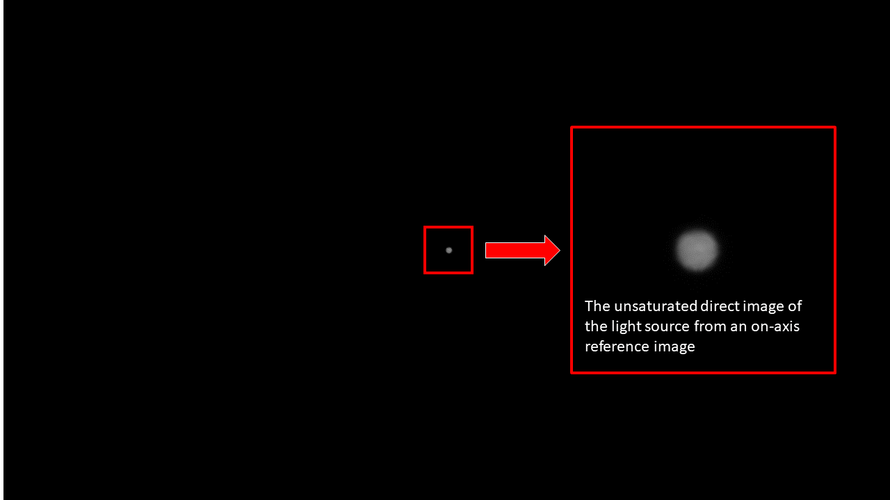
Figure 2: An on-axis reference image showing an unsaturated direct image of the light source. The image was captured using a shorter camera exposure time than the test images and with an ND 2.5 filter in front of the light source. In the separate test images (not shown), the direct image of the source is saturated and significantly blooming to reveal stray light.
References
[1] B. Bouce, et. al, 1974. “GUERAP II – USER’S GUIDE”. Perkin-Elmer Corporation. AD-784 874.
[2] Jackson S. Knappen, “Comprehensive stray light (flare) testing: Lessons learned” in Electronic Imaging, 2023, pp 127-1 – 127-7, https://doi.org/10.2352/EI.2023.35.16.AVM-127