Imatest’s charts and software allow you to measure the characteristics and parameters of imaging systems. Quite often these measurements simply indicate the limits of system performance and expected image quality.
But some Imatest results let you improve image quality— and subsequent images taken by the same system— by correcting measured aberrations. No new components need to be purchased; no judgement calls need to be made. All it takes is some math and computation, which you can apply in our own external program or with an Imatest module. This is an aspect of image processing pipeline tuning, which is usually done by a dedicated Image Signal Processing (ISP) chip in a device to transform raw sensor data into an appropriate image.
At Imatest, we informally call this “closing the loop”, because it completes the cycle from the camera-under-test to measurement, back to the camera (in the form of an adjustment).
Today, we’re going to illustrate how to use radial distortion measurements from Imatest to correct for optical distortion (without buying a new lens).
Radial Geometric Distortion
Geometric distortion, for the purposes of this post, is roughly defined as the warping of shapes in an image compared to how those shapes would look if the camera truly followed a simple pinhole camera model. (Consequently, we’re not talking here about perspective distortion). The most obvious effect of this is that straight lines in the scene become curved lines in the image.
Geometric distortion is not always a bad thing- sometimes curvilinear lenses are chosen on purpose for artistic effect, or a wide angle lens is used and the distortion is ignored because that’s what viewers have come to expect from such situations. However, subjective user studies have shown that the average viewer of everyday images has limits on the amount of distortion they are willing to accept before it reduces their perception of image quality.
Characterizing (and correcting for) distortion is also necessary for more technical applications which require precise calibration, such as localization of a point in 3-D space in computer vision or for stitching multiple images together for panoramic or immersive VR applications.
This geometric distortion is almost always due to lens design, and because of that (and how lenses are constructed), it is typically modeled as being (1) purely radial and (2) radially symmetric.
Purely radial distortion means that no matter where in the image field we consider a point, the only relevant aspect of that point for determining the distortion it has undergone is how far from the center of the image it is. (For the sake of simplicity, we will assume here that the center of the image is the optical center of the system, though in general this needs to be measured in conjunction with or prior to radial distortion.) Assuming geometric distortion is radial is extremely helpful in reducing the complexity of the problem of characterizing it, because instead of a 2-dimensional vector field over two dimensions (x- and y- displacement at each pixel location) we only have to determine a 1-dimensional over one dimension (radial displacement at each radius).
By using the SFRPlus, Checkerboard, or Dot Pattern modules, Imatest can measure radial distortion in a camera system from an image of the appropriate test charts.
Distortion Coefficients in Imatest
Imatest can return functional descriptions of two different types of radial distortion. Both are described by polynomial approximations of the distortion function, but the two polynomials represent different things. In many cases, they are functionally equivalent and one can convert from one form function to the other. (For simplicity, we ignore here the tan/arctan approximation Imatest can provide and note that when it comes to distortion correction it can be applied in the same way with a change only to the forward mapping step.)
In the rest of this post, we will use the following conventions:
- \(r_d\) is the distorted radius of a point, i.e. its distance from center in the observed (distorted) image
- \(r_u\) is the undistorted radius, of the point, the distance from center it would have appeared at in an undistorted image
- The function \(r_d = f(r_u)\) is called a forward transformation because it takes an undistorted radius value and converts it to a distorted radius. That is, it applies the distortion of the lens to the point.
- The function \(r_u = f^{-1}(r_d)\) is called an inverse transformation because, in contrast to a forward transformation, it undoes the distortion introduced by the lens.
- \(P(\cdot)\) indicates a polynomial function
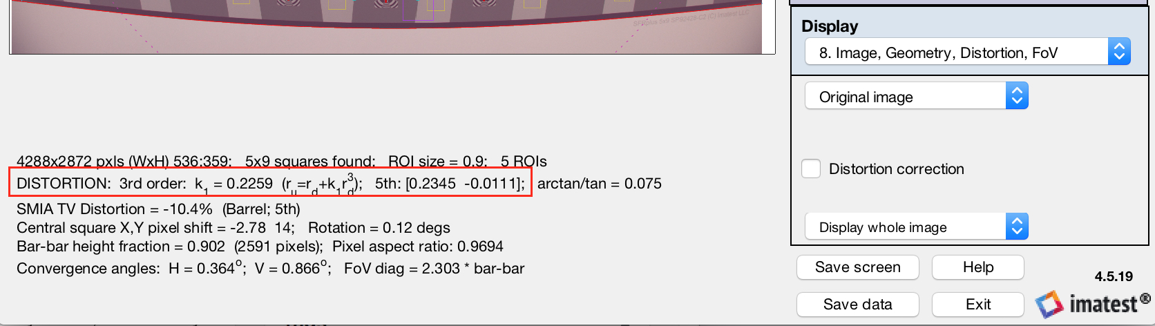
SFRPlus and Checkerboard modules return the polynomial coefficients that describe the inverse transformation which corrects the distortion, \(r_u = f^{-1}(r_d)\), highlighted in Rescharts below.
Dot Pattern module returns the polynomial coefficients for a different parameterization of radial distortion, known as Local Geometric Distortion (LGD), or sometimes known as optical distortion. This is the description of radial distortion used by the standards documents of ISO 17850 and CPIQ.
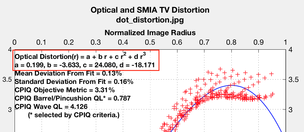
LGD is defined as the radial error relative to the true error, as a percentage (i.e., multiplied by 100):
\[LGD = 100*\frac{r_d – r_u}{r_u}\]
By considering LGD to be a polynomial function of radius in the distorted image, \(P(r_d)\), we can re-arrange the sides of this equation to yield a more useful equation, a rational polynomial form of a distortion-correcting inverse transformation. Thus the dot pattern results can be used in the same way as the SFRPlus/Checkerboard results (though we will be be directly replacing this rational polynomial with a regular polynomial fit approximation in the code example).
\[r_u = \frac{r_d}{P(r_d)/100 + 1} = f^{-1}(r_d)\]
Distortion Correction by Re-Sampling
The pixel array of an image sensor essentially takes a grid of regularly-spaced samples of the light falling on it. However, the pattern of light falling on it has already been distorted by the lens and so while the sensor regularly samples the light this light, these are effectively not regular samples of the light as it appeared before entering the lens. Our computational solution for remedying this can be described as follows:
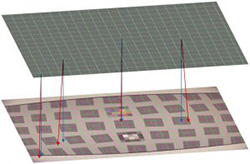
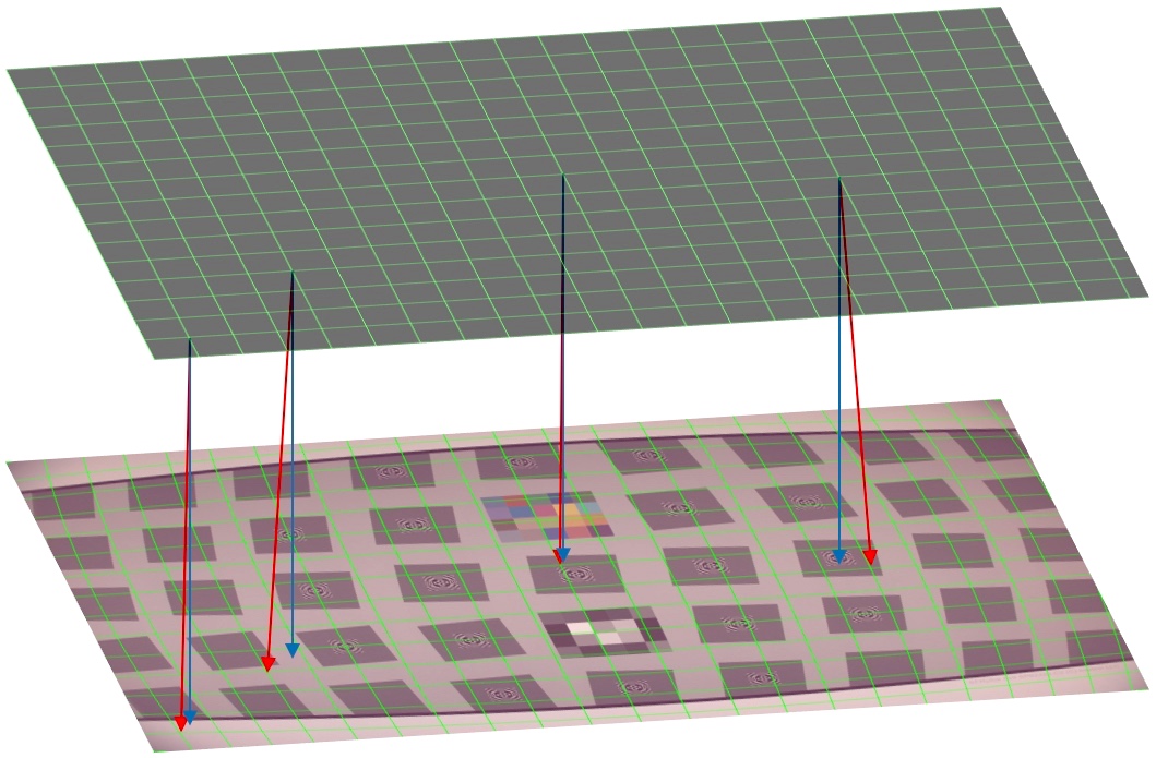
We create a new undistorted, regularly spaced grid (a new array of pixels). At each of those “virtual sensor” pixel locations we re-sample image data from the observed image at the location in that image where the sensor pixel would have projected in the absence of distortion. So the distorted image is re-sampled by a grid which undergoes the same distortion, but the sampled results are then presented regularly spaced again- effectively undoing the distortion. This is illustrated below.
Each of the intersection points of the upper grid lines represents a pixel location in our generated, undistorted image (the pixel locations in our “virtual sensor”). Obviously, we have reduced the number of “pixels” here to increase legibility. The lower part of the image represents the distorted image with the sampling grid overlaid on it after the grid has been distorted the same way. The regularly spaced array locations above will be populated with data sampled irregularly from the distorted image below, as indicated by the distorted grid intersection locations.
As a further visual aid, the red arrows descend from the grid intersections in the upper image to the corresponding grid intersections in the lower one. These can be contrasted to the ending locations of the blue arrows, which indicate there the pixel samples would be if undistorted. (Obviously, if the pixel sample locations were not distorted, i.e. the blue arrow locations were used, then the output image would be sampled regularly from the distorted image, and would itself be distorted.)
An Example
The following example of how to do this re-sampling is provided in MATLAB code, below. You can also download the code and example images at the bottom of this post. The code is merely a particular implementation, though- the concepts can be extracted and applied in any programming language.
Note that below, we use the convention of using suffixes ‘_d’ and ‘_u’ to identify variables which are related the distorted and undistorted images/coordinates respectively, and use capitalized variables, such as RHO, to identify matrices of the same size as the test and output images (a property that will be used implicitly below).
(0) Load the image of an SFRPlus chart into Imatest and analyze it to determine the inverse transformation coefficients (shown here measured in the Rescharts interactive module). (Alternatively, load an image into Dot Pattern module and retrieve the LGD coefficients from there and convert them into inverse transformation coefficients, and then follow along with the remaining steps.) Load these into MATLAB.

inverseCoeffs = [0.2259 0 1 0]; % distortion coefficients reported by SFRPlus
im_d = double(imread('sfrplus_distortion.jpg'));
width = size(im_d, 2);
height = size(im_d, 1);
channels = size(im_d, 3);
(1) Define the spatial coordinates of each of the pixel locations of this observed (distorted) image, relative to the center of the image. For example, since this test image is 4288×2872 pixels, the upper left pixel coordinate is (-2143.5, -1435.5).
xs = ((1:width) - (width+1)/2);
ys = ((1:height) - (height+1)/2);
[X, Y] = meshgrid(xs,ys);
(2) Convert these coordinates to polar form so we can manipulate only the radial components (called RHO here). We also normalize and then scale the radial coordinates so that the center-to-corner distance of the undistorted image will ultimately be normalized to 1.
[THETA, RHO_d] = cart2pol(X, Y);
normFactor = RHO_d(1, 1); % normalize to corner distance 1 in distorted image
scaleFactor = polyval(inverseCoeffs, 1); % scale so corner distance will be 1 after distortion correction
RHO_d = RHO_d/normFactor*scaleFactor;
(3) NOTE: As a subtle point, the pair of variables THETA and RHO_d actually define spatial coordinates two ways: explicitly and implicitly. They define explicit coordinates in their values, i.e. in that (THETA(1,1), RHO(1,1)) defines the angular and radial coordinate of the upper left corner pixel of the image. However, they also implicitly define a set of coordinates simply by being 2-D arrays, which have a natural ordering and structure. Even if we change the value of the (1,1) entry of these two arrays, they are both still the upper left corner entry of each array. The explicit coordinate of the point has changed, but the implicit one has remained the same.
We now apply the measured distortion to the radial coordinates, so that the explicit radial distance matches the radial distance of that point in the observed image. As pointed out above, this distorted location in the observed image is now tied to the undistorted location in the image array via the implicit location in the array. We are using the implicit array element locations as the true coordinates of the undistorted image, and the explicit array values as a map to the point in the distorted image to pull the samples from.
Note that we don’t actually have the forward transformation polynomial yet, we have the inverse polynomial as returned by Imatest. This can be inverted by fitting a new (inverse of the inverse) polynomial, as in the provided invert_distortion_poly.m file.
forwardCoeffs = invert_distortion_poly(inverseCoeffs);
RHO_u = polyval(forwardCoeffs, RHO_d);
% Convert back to cartesian coordinates so get the (x,y) distorted sample points in image space
[X_d, Y_d] = pol2cart(THETA, RHO_u*normFactor);
(4) We now have X_d, Y_d arrays whose implicit coordinates are those of the undistorted image and whose explicit values indicate the sampling points in the observed image associated with them. We can use these directly as query (sampling) points in the interp2() function.
% Re-sample the image at the corrected points using the interp2 function. Apply to each color
% channel independently, since interp2 only works on 2-d data (hence the name).
im_u = zeros(height,width,channels); % pre-allocate space in memory
for c = 1:channels
   im_u(:,:,c) = interp2(X, Y, im_d(:,:,c), X_d, Y_d);
end
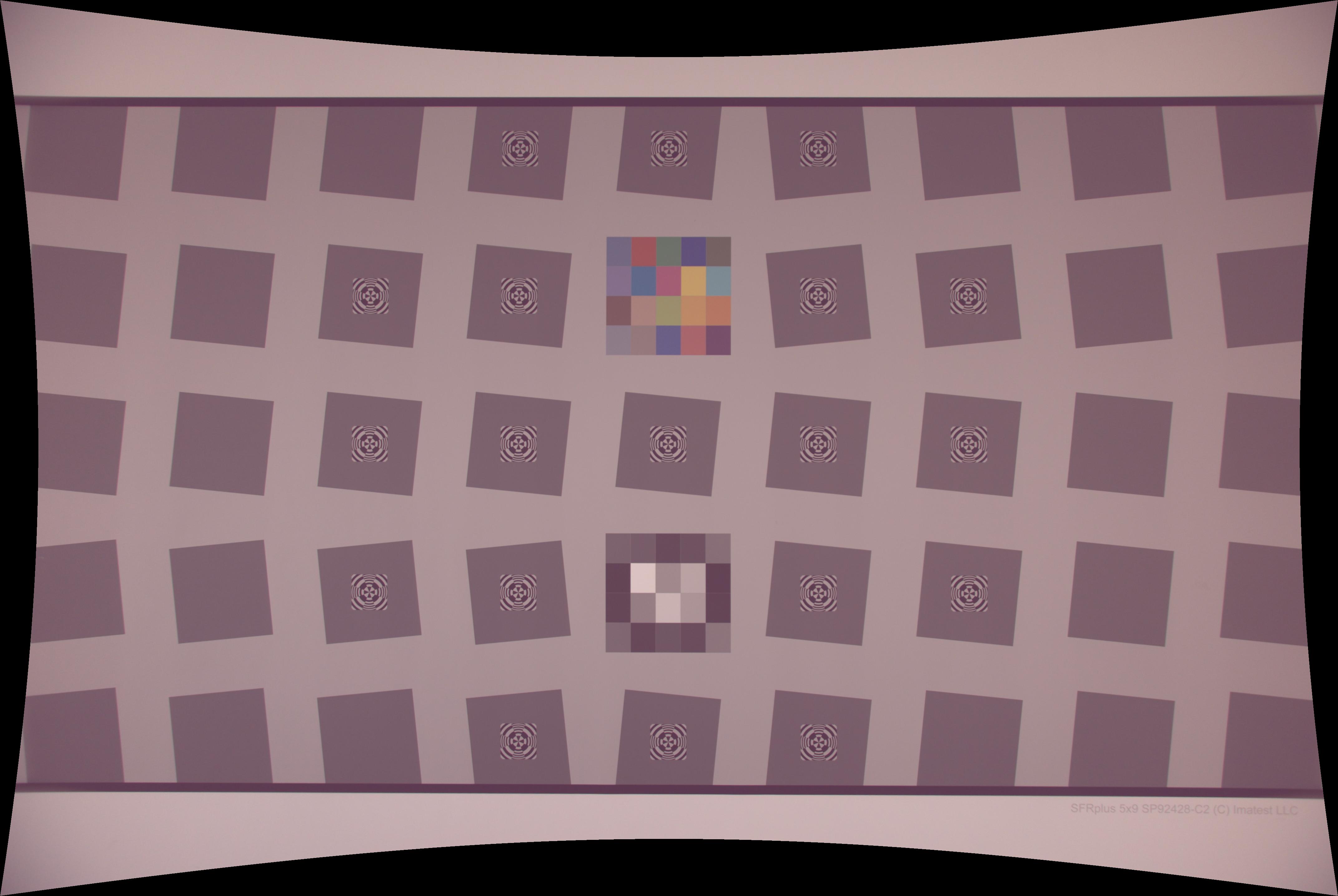
That’s it! Now we can view the undistorted fruits of our labor. Notice the straightened lines on top and bottom, in particular. Also note that there are black areas around the edges of this undistorted image- of course, there was no information in the original image to use to meaningfully fill in there.
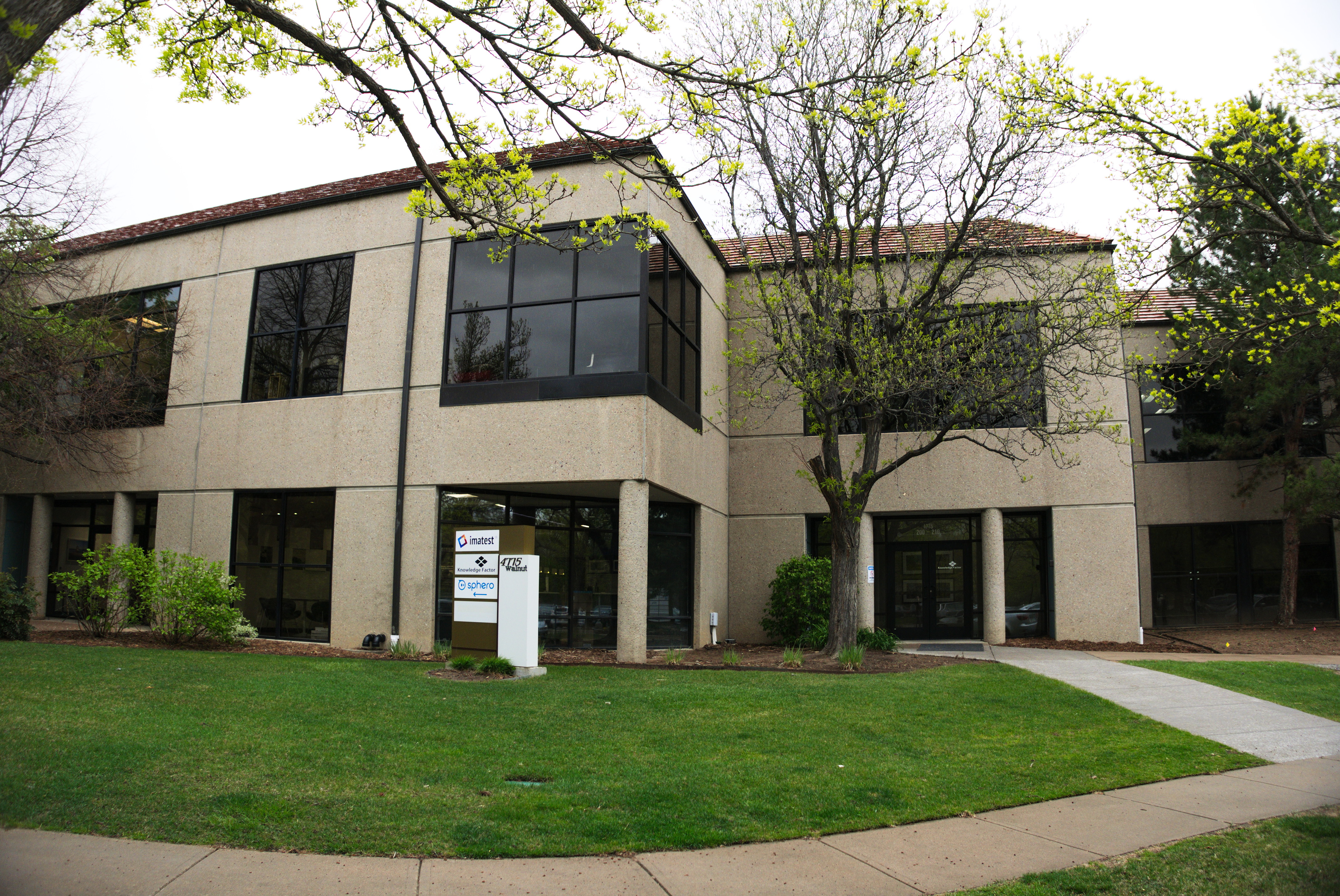
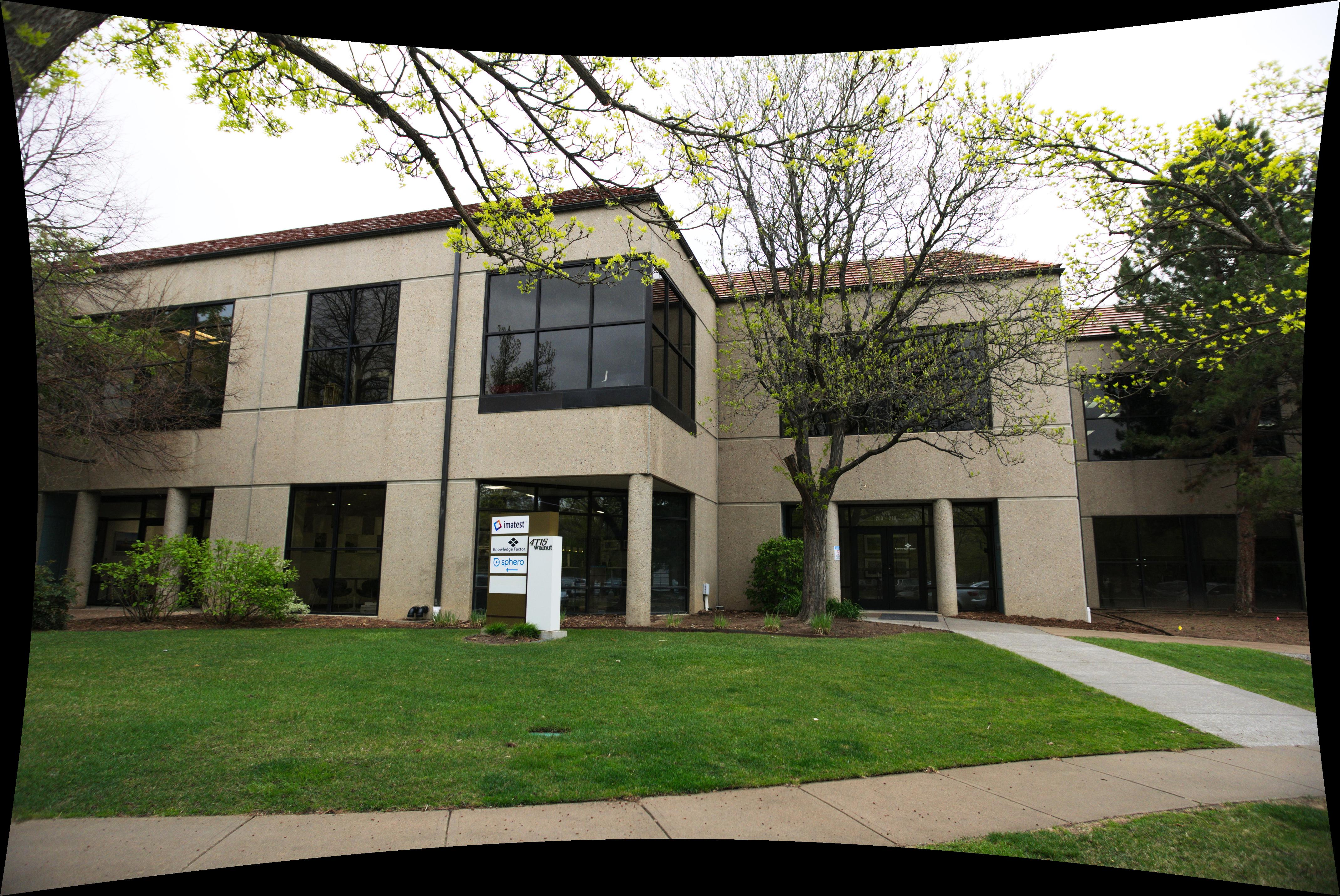
Of course, we can now undistort scenes besides just test chart images. Now that we have used the test chart and Imatest to characterize the distortion caused by the camera system itself, we can undo that distortion in any other image it takes. Since the supposed-to-be-straight lines of architecture are a very common source of noticeable distortion, we demonstrate this on a photo of our office building in Boulder, CO on a day with diffuse lighting (i.e., gloom).
These example images and a more verbose version of the MATLAB code are available here – distortion_correction_example.zip 5.4 MB
You can measure the distortion in the images yourself in Imatest, or use the supplied values in the distortion_correct_ex.m file. We hope that this post has helped illustrate how this Imatest measurement can be immediately useful for incorporating into your pipeline to improve your images.
The Imatest Radial Geometry module (added to Imatest 5.0, August 2017)
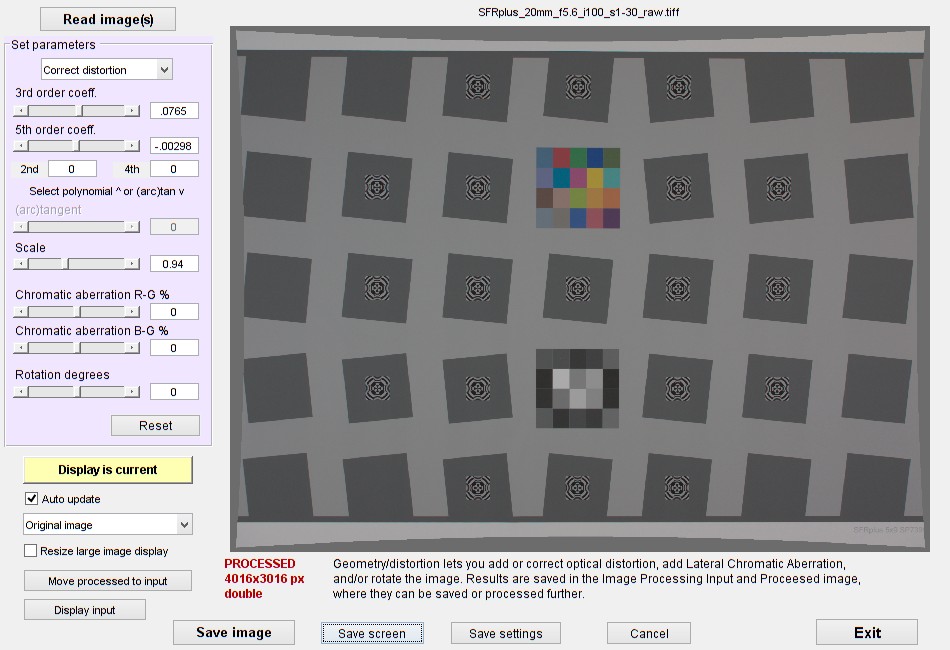
If you don’t want to code your own, you can add or correct distortion using the Radial Geometry module, which works on single images or batches of images (using settings from the most recent single image run). Full details, including a description of the settings, are in the Radial Geometry instructions.
Here is the input window after reading a distorted image of an SFRplus test chart image.
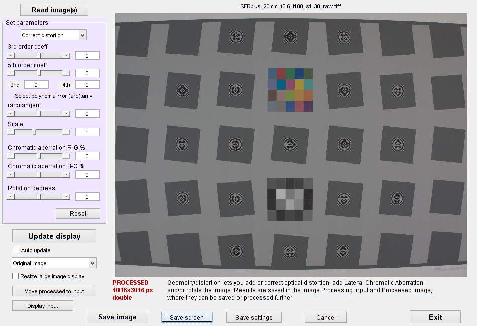 Radial Geometry opening window.
The image is from a dcraw-converted image (with no distortion-correction).
Parameters may be obtained from Imatest runs: SFRplus is shown in the following example.
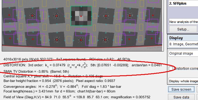 SFRplus Setup results for above image, showing distortion calculations
Here is the corrected result.
 Corrected image using parameters from SFRplus Setup
