Author: Henry Koren
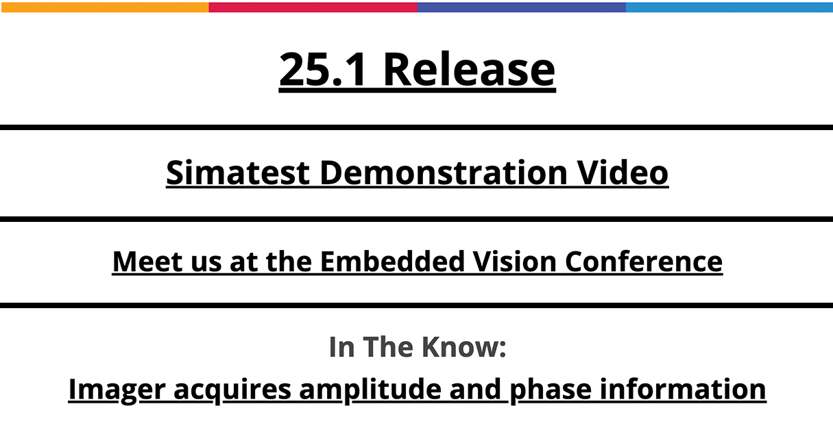
Imatest Releases Version 25.1
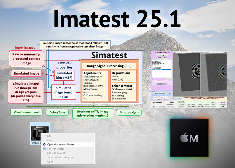
Simatest Camera & ISP Simulator, Open With Imatest, UI & Settings Improvements, Output Documentation
Validating Information Metrics Correlation with Object Detection
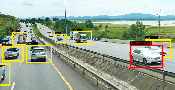
Update: the contents of this post led to the publication of this paper: D. Geever, T. Brophy, D. Molloy, E. […]
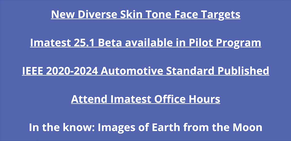
Improving Image Equity: Representing diverse skin tones in photographic test charts for digital camera characterization
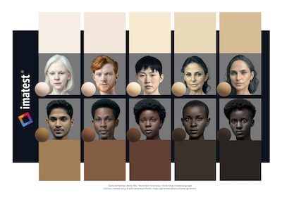
Megan Borek; Imatest LLC; Boulder, CO, USA This paper was presented on 2025-02-05 at Electronic Imaging 2025 Abstract: Accurate representation […]

2024 Year In Review
In 2024, Imatest greatly increased our image quality testing capabilities with significant advancements across software, hardware, charts, and solutions. We […]
Imatest releases version 24.2
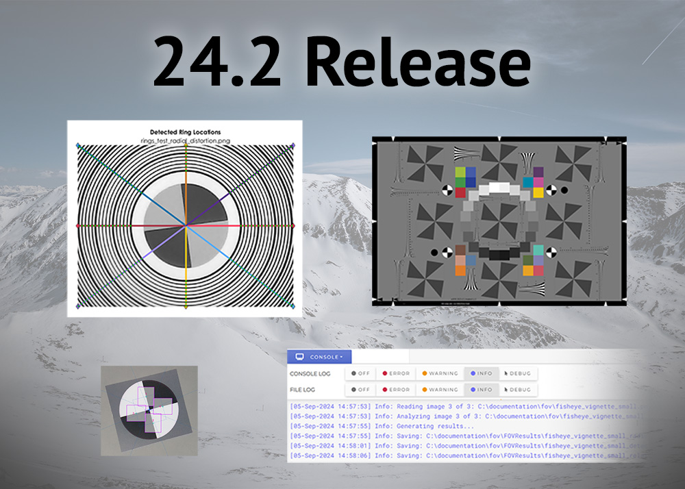
Concentric ring FOV, ISO Sharpness target support, batch folder processing, console panel, macOS Sequoia
Imatest 20th Anniversary
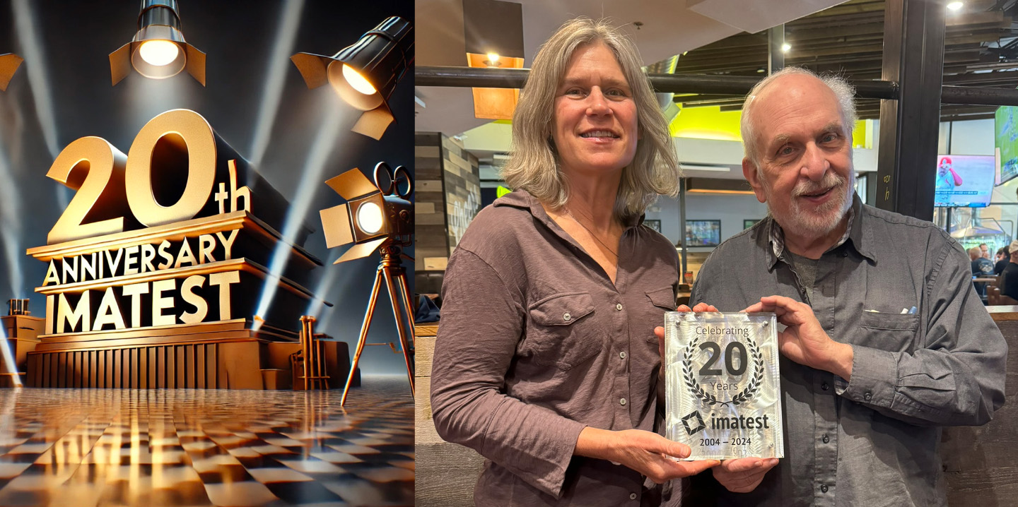
Imatest was founded by Norman Koren in Boulder, Colorado, in 2003. On September 4th 2004, we sold our first Imatest 1.0 licenses. […]
AutoSens Europe 2024
Join us and other automotive imaging industry experts on October 8-10 in Barcelona, Spain. We will present our advanced testing methods and algorithms […]
Using Imatest with CODE V 2D Image Simulation (IMS)
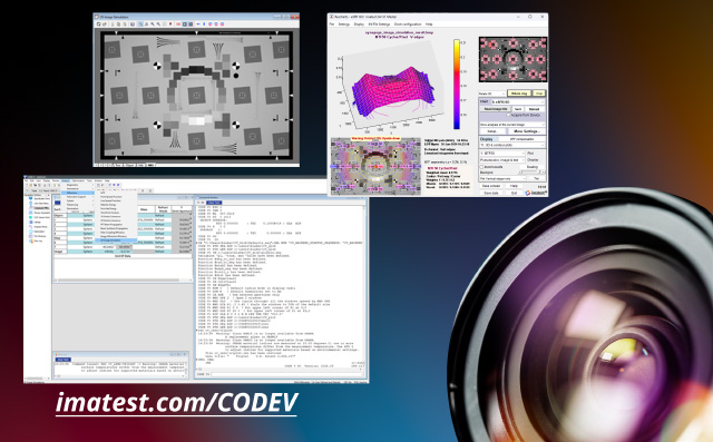
Imatest test charts raster files and can be used with 2D Image Simulation (IMS) to create images with the degradations […]
Photometry Luminance and Illuminance units vs. Radiometry Radiance and Irradiance units
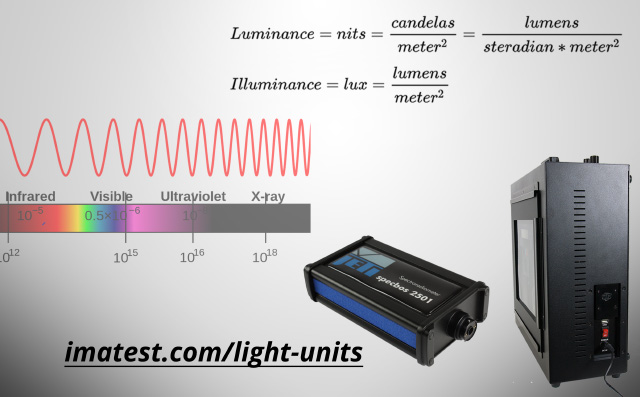
This knowledge base post describes why lightboxes are traditionally described in photometric illuminance units of Lux, despite a more appropriate […]
Imatest release new version Imatest 24.1
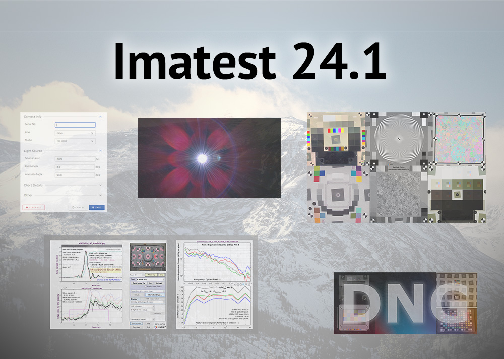
Custom Metadata, Edge Informatiom Metrics, DNG improvements, Stray Light improvements & Registration Mark Detection.
Imatest Presented at AutoSens USA 2024
Leader SFR-Fit MTF Measurement Software SFR-Fit is camera resolution measurement software that measures MTF (Modulation Transfer Function). MTF indicates spatial […]
Imatest Electronic Imaging 2024 Recap
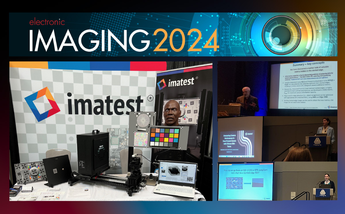
Have a virtual visit to our booth and read the papers we published to advanced imaging science.
Test Lab Services Drone Comparison
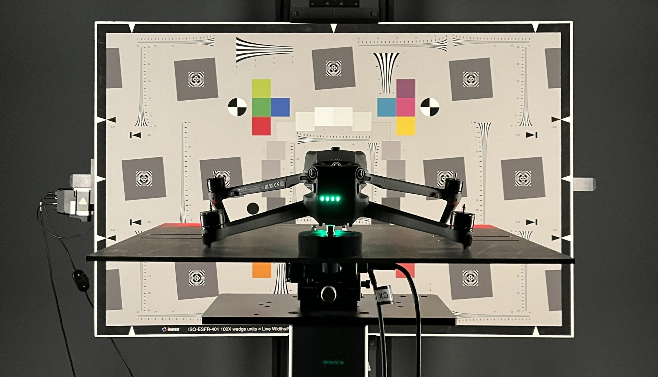
Skydio reached out to Imatest for an independent, objective comparison of different manufacturers’ drones. Our focus was on critical aspects […]