Imatest not vulnerable to Apache log4j security compromise

Security researchers disclosed the following vulnerabilities in the Apache Log4j Java logging library:

  • CVE-2021-44228: Apache Log4j2 JNDI features do not protect against attacker-controlled LDAP
    and other JNDI related endpoints
  • CVE-2021-45046: The fix for CVE-2021-44228 was incomplete in certain non-default
    configurations.
  • CVE-2021-45105: Apache Log4j2 Context Lookup features do not protect against uncontrolled
    recursion from self-referential lookups in certain non-default configurations

No Imatest software includes the affected versions of Log4j, no dependency used, such as the MATLAB compiler runtime includes an affected version either.

Internal Imatest systems which included Log4j were promptly patched when the vulnerability was discovered. These were never publically accessable.

Thank you for your concern.

Read More

Test Chart Life Span

 Best storage practices would be in a clean, dark, dry area at (~ 23°C / 72°F) or below.  Exposure to UV will break down pigments and cause loss of contrast and saturation.

Color Test Charts

Such as X-Rite colorcheckers.  Certified to last two years if stored properly.  You can use a spectrophotometer to generate a reference file for an older/faded chart.

Color LVT Film

The main factors affecting the films are humidity and UV light.

If the chart is used heavily (exposed to light every day) it can last up to one year.

If they are stored dark place and not used very often they can last up to 5 years.

Significant heat exposure ( > 52°C / 125°F) will decouple the dyes and significantly hasten the fading time.


Read More

Logarithmic wedges: a superior design

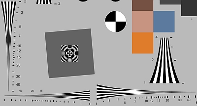
We introduce the logarithmic wedge pattern, which has several advantages over the widely-used hyperbolic wedges found in ISO 12233 (current and older) and eSFR ISO charts.

The key advantage of logarithmic wedges is that charts with large fmax/fmin ratios work well for systems with a wide range of resolutions, unlike hyperbolic wedges, where large ratios cause high frequencies occupy excessive real estate and low frequencies to become highly compressed. The fmax/fmin ratio of the hyperbolic wedges in the ISO 12233/2017 chart is only 12.5:1 — insufficient for modern high resolution cameras.

(more…)

Read More

Imatest Releases Version 2021.2

Imatest Version 2021.2 introduces our new Main Window User Interface, File First Workflow, Dark Mode, a new ‘Learn’ Function, Distortion Contour Plots for Checkerboard Output, new JSON output fields, and more. (more…)

Read More

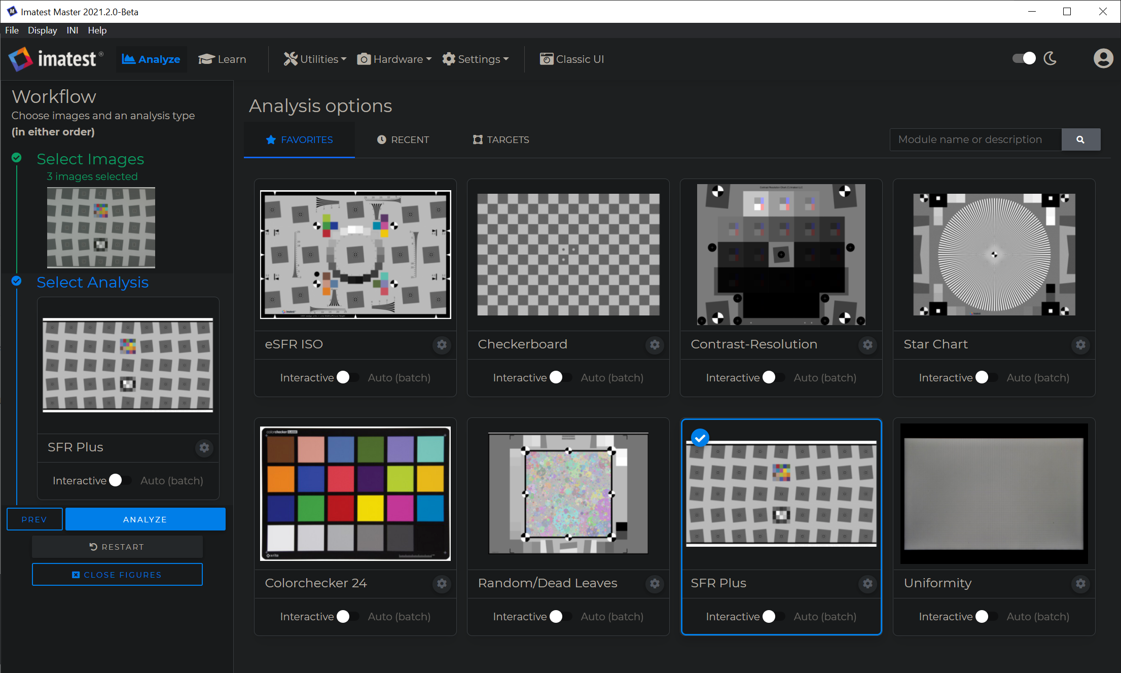
How to compute resolution in TV Lines (TVL)

Television Lines (TVL) are derived from the EIA 1956 testing standard, where they are defined as the number of light and dark vertical lines that are visible (i.e., distinguishable) over the height of the screen. TVL defines “lines” as distinct dark and light lines. This is equivalent to Line Widths (LW), and should not to be confused with Line Pairs (LP), which represent a complete cycle, i.e., one TV line is equivalent to half a line pair. Although TVL is not the best measurement of digital imaging system quality, it can be useful for comparing digital systems with older analog systems.

The definition of TVL is problematic because “resolved” or “visible” are not clearly defined. There is no description of the viewing conditions, no objective definition of the contrast representing “light” and “dark”, and no description of how much contrast is lost before detail is considered “no longer resolved”.  Is a 90% loss of the signal (MTF10) enough to be considered “no longer resolved?”  This is a relatively common definition of resolution (derived from the Rayleigh diffraction limit), and it has been standardized for Camera Monitor Systems in the ISO 16505:2015 standard.  We have proposed an improved definition of resolution, but it has only gained limited traction. Using wedge patterns, some observers state that lines can no longer be resolved at 70% (MTF30) or 80% (MTF20) loss of contrast. Relying on subjective assessment of observers makes it difficult to get a consistent objective definition of TV lines.

TVL measurements do not consider changes in sharpness across the image that are typical of conventional lenses. Measuring the center-only may produce optimistic results. The EIA 1956 and ISO-12233:2000 charts had wedges in the corners that were easy to ignore. You should consider points all across the image to get a full understanding of your system’s resolution. You can use a mean of these values if you only want a single number. Remember that the tilt of your lens can degrade resolution in some corners, but boost it in opposite corners, without having much effect on the mean MTF.

A convenient, stable method of measuring TV lines in displays (i.e.,monitors) is given in Display (Monitor) Sharpness. For most other images we recommend using MTF20 (or better, MTF20P) in units of LW/PH (Line Widths per Picture Height), measured with (near) vertical slanted edges. (MTF20P is less sensitive than MTF20 to excessive software sharpening.)

note: for cropped images enter the original picture height into the more settings dimensions input.

If you can control the processing of your imaging system so you can disable sharpening or analyze unsharpened RAW images, you can make an approximate TVL measurement using “MTF10 LW/PH” or “MTF20 LW/PH” from vertical edges across the image. You can use the Multi-region summary plot from SFR, SFRplus, eSFR ISO, Checkerboard, or SFRreg modules to obtain a weighted mean MTF10 or MTF20 in LW/PH units, which are good objective approximations to the TVL metric. This is superior to the wedge measurement described below since it is less affected by aliasing, but it may not be the best measurement if you cannot disable your cameras sharpening.
 
If you have a “black box camera” system where you cannot disable sharpening, we recommend the hyperbolic wedge pattern to measure high-frequency MTF or vanishing resolution. Otherwise, the slanted edge MTF10 or MTF20 numbers may be exaggerated by the sharpening. Our best target for measuring multiple wedges across the field is our ISO 12233:2017 target with “extra wedges”. The best Output is our Multi-Wedge plot. The Weighted Mean Wedge MTF10 or MTF20 in units of LW/PH is very close to TV Lines.

Read More

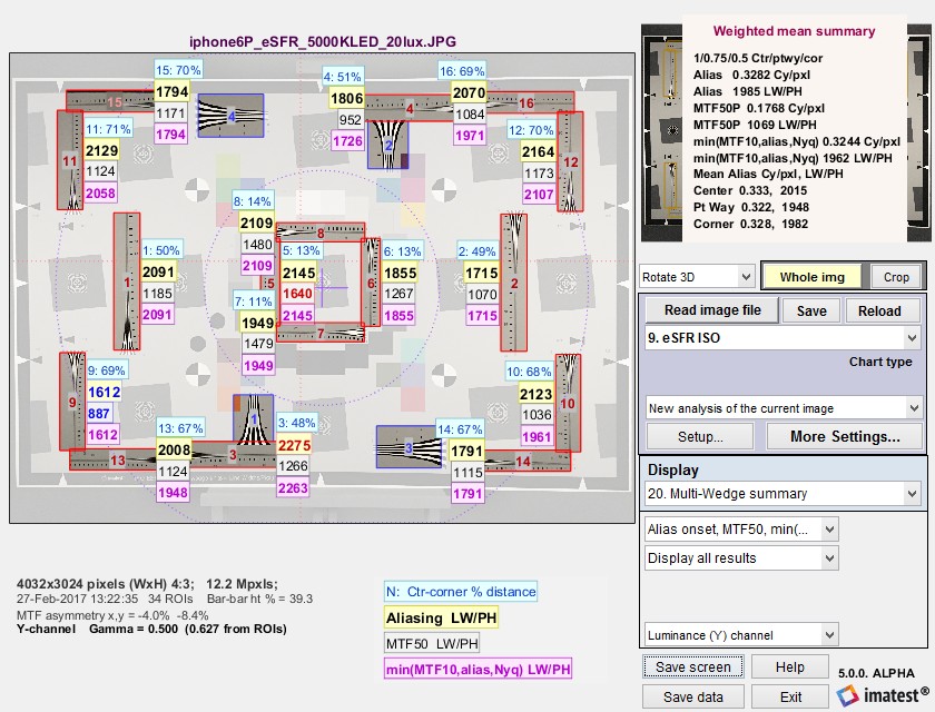
Interactive vs. Auto(Batch) Analyses

Imatest has two types of analysis module: Fixed (in the left-most column of the main window) and Interactive (in the second column).
  • Fixed modules require that all settings be entered prior to running the analysis. Stored settings are read from imatest.ini and can be changed by user input. Results are displayed as figures and can be saved as image (usually PNG), CSV, XML, and JSON files.
     
  • Interactive modules are run from GUIs (Graphic User Interfaces) that allow results to be queried and modified after the analysis has been run. This allows you to explore results in great depth. Results can be saved as image (usually PNG), CSV, XML, and JSON files.
Auto(Batch) / Fixed vs. Interactive module summary
Auto(Batch) / Fixed Interactive
Graphic results in Figures allow limited manipulation (zooming or rotation for 3D images). Graphic results displayed in GUI windows allow a high degree of manipulation: You can change calculation and display settings and you can select any available display. You can analyzed results in great depth.
Batches of files can be run. Only a single file can be analyzed (one exception: several files can be combined (signal-averagted) to improve signal-to-noise ratio (SNR)).
Most are available as Industrial Testing (IT) modules (EXE or DLL programs that can run in production/quality control environments). Not directly available in IT.
Images cannot be directly acquired (in the Image Sensor edition). In the Imatest Image Sensor Edition, Images can be acquired directly from devices (development boards from Aptina, Omnivision and others as well as devices supported by the Matlab Image Acquisition toolbox). Directly-acquired images can be continuously refreshed in realtime.


In most (but not all) cases there are corresponding Fixed and Interactive modules.


Coresponding Interactive and Auto(Batch) / Fixed modules
Interactive module
Auto(Batch) / Fixed module
Notes
Rescharts

Interactive interface for several separate sharpness modules.

SFRplus Auto All settings must be made in Rescharts (SFRplus Setup). SFRplus Auto is highly automated (with automated region detection based on criteria set in Rescharts), requiring no user input.
SFR Fixed SFR can analyze several regions (ROIs); Rescharts SFR can only analyze a single region.
Random/Dead Leaves  
Log F-Contrast  
Star  
Wedge  
Any image sharpness  
Multicharts

Analyze color/grayscale charts.

ColorTest Can analyze a large variety of color charts, including the Colorchecker 24-patch and SG, the DSC Labs ChromaduMonde, the IT8.7, and many others (all charts supported by Multicharts). Before running ColorTest, the chart type should be selected in ColorTest settings (in the Fixed Modules or Settings dropdown menus). Plots are identical to Multicharts. There is considerable overlap with Stepchart and Colorcheck, both of which were developed earlier.
Stepchart Can analyze a large variety of grayscale stepcharts, including the Q-13/Q-14, ISO-14524, ISO-15739, Imatest 36-patch Dynamic Range chart, and many others. Figures are slightly different from Multicharts, but Multicharts chart seleections 6. Grayscale Stepchart (linear) and 7. Special Grayscale & Color charts correspond to charts supported by Stepchart.
Uniformity Interactive Uniformity Settings made in either module are used by the other. Blemish Detect capability is not yet included in Uniformity Interactive, but Blemish (fixed module) has most Uniformity functions.


Read More

Camera to Chart Alignment

Centering test charts is critical for image quality testing. If the camera is not properly aligned with the test chart, your image may not be suitable for analysis; you may not know if the results are truly indicative of the camera system, or from an error in positioning the chart.  (more…)

Read More

Long Range Testing with the OSCM10120 Target Projection Collimator

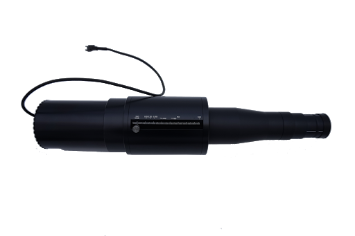
Introducing the CM10120 Collimator – a target projection collimator system that allows users to simulate long-range testing in confined spaces. This compact solution can be used for regional sharpness testing, making it useful for tasks such as setting focus or checking pass/fail criteria. The CM10120 includes adjustable distance simulation and is suitable for R&D, production, and end of line testing. To learn more about the CM10120contact us at sales@imatest.com.

Read More

Gamma, Tonal Response Curve, and related concepts

IntroductionEncoding vs. Display gammaWhy logarithms? 
How gamma-encoding increases dynamic range – Expected gamma valuesGamma and MTF 
Which patches are used to calculate gamma? – Why gamma ≅ 2.2?Why are raw-converted images often dark? 
Tone mappingContrast definitions: Ratio, Weber, MichelsonLogarithmic color spacesMonitor gamma 

Introduction

In this post we discuss a number of concepts related to tonal response and gamma that are scattered around the Imatest website, making them hard to find. We’re putting them together here in anticipation of questions about gamma and related concepts, which keep arising.

Gamma (γ) is the average slope of the function that relates the logarithm of pixel levels (in an image file) to the logarithm of exposure (in the scene).

\(\text{log(pixel level)} \approx  \gamma \ \text{log(exposure)}\)

This relationship is called the Tonal Response Curve, (It’s also called the OECF = Opto-Electrical Conversion Function). The average is typically taken over a range of pixel levels from light to dark gray.

Tonal Response Curve for Fujichrome Provia 100F film. The y-axis is reversed from the digital plots.

Tonal Response Curves (TRCs) have been around since the nineteenth century, when they were developed by Hurter and Driffield— a brilliant accomplishment because they lacked modern equipment. They are widely used for film. The Tonal Response Curve for Fujichrome Provia 100F film is shown on the right. Note that the y-axis is reversed from the digital plot shown below, where log(normalized pixel level) corresponds to \(D_{base} – D\text{, where } D_{base} = \text{base density} \approx 0.1\). 

Equivalently, gamma can be thought of as the exponent of the curve that relates pixel level to scene luminance.

\(\text{pixel level = (RAW pixel level)}^ \gamma \approx \text{exposure} ^ \gamma\)

There are actually two gammas: (1) encoding gamma, which relates scene luminance to image file pixel levels, and (2) display gamma, which relates image file pixel levels to display luminance. The above two equations (and most references to gamma on this page) refer to encoding gamma. The only exceptions are when display gamma is explicitly referenced, as in the Appendix on Monitor gamma.

The overall system contrast is the product of the encoding and decoding gammas. More generally, we think of gamma as contrast.

Encoding gamma is introduced in the image processing pipeline because the output of image sensors, which is linear for most standard (non-HDR) image sensors, is never gamma-encoded. Encoding gamma is typically measured from the tonal response curve, which can be obtained photographing a grayscale test chart and running Imatest’s Color/Tone module (or the legacy Stepchart and Colorcheck modules).

Display gamma is typically specified by the color space of the file. For the most common color space in Windows and the internet, sRGB, display gamma is approximately 2.2. (It actually consists of a linear segment followed by a gamma = 2.4 segment, which together approximate gamma = 2.2.) For virtually all computer systems, display gamma is set to correctly display images encoded in standard (gamma = 2.2) color spaces. 

Here is an example of a tonal response curve for an in-camera JPEG for a high quality consumer camera, measured with Imatest Color/Tone.

Tonal response curve measured by the Imatest Color/Tone module
from the bottom row of the 24-patch Colorchecker,

Note that this curve is not a straight line. It’s slope is reduced on the right, for the brightest scene luminance. This area of reduced slope is called the “shoulder”. It improves the perceived quality of pictorial images (family snapshots, etc.) by reducing saturation or clipping (“burnout”) of highlights, thus making the response more “film-like”. A shoulder is plainly visible in the Fujichorme Provia 100D curve, above. Shoulders are almost universally applied in consumer cameras; they’re less common in medical or machine vision cameras.

Because the tonal response is not a straight line, gamma has to be derived from the average (mean) value of a portion of the tonal response curve. 

Why use logarithms?

Logarithmic curves have been used to express the relationship between illumination and response since the nineteenth century because the eye’s response to light is logarithmic. This is a result of the Weber-Fechner law, which states that the perceived change dp to a change dS in an initial stimulus S is

\(dp = dS/S\)

Applying a little math to this curve, we arrive at \(p = k \ln(S/S_0)\)  where ln is the natural logarithm (loge).

From G. Wyszecki & W. S. Stiles, “Color Science,” Wiley, 1982, pp. 567-570, the minimum light difference ΔL that can be perceived by the human eye is approximately

\(\Delta L / L = 0.01 = 1\% \). This number may be too stringent for real scenes, where ΔL/L may be closer to 2%.

How gamma encoding increases Dynamic Range

In photography, we often talk about zones (derived from Ansel Adams’ zone system). A zone is a range of illumination L that varies by a factor of two, i.e., if the lower and upper boundaries of a zone are L1 and L2, then L2 /L1 = 2 or log2(L2) – log2(L1) = 1.

1 2 3 4 5 6 7 8 9


Zone system chart for gamma = 2.2 (sRGB color space, etc.)

The steps between each zone has equal visual weight, except for very dark zones where the differences are hard to see.

For a set of zones z = {1, 2, 3, ..} the relative illumination of zone n is 2-(z-1) = {1, 0.5, 0.25, 0.125, …}. The illumination difference between zones is {0.5, 0.25, 0.125, …}. The scene illumination ratio is always 2:1.

Geek alert: a lot of numbers follow— all of which are intended to show how gamma encoding increases the effective dynamic range.

The total number of available pixel levels B is a function of the bit depth, B = 2(bit depth). For bit depth = 8, B = 256; for bit depth = 16, B = 65536. The relative pixel level of zone n for encoding gamma γe is bn = B × 2-(n-1)γe.For linear gamma (γe = 1), bn= {1.0, 0.5, 0.25, 0.125, …} (the same as L). For γe= 1/2.2 = 0.4545, bn = {1.0000, 0.7297, 0.5325, 0.3886, 0.2836, 0.2069, 0.1510 ,0.1102, …}. The relative pixel levels bn decrease much more slowly than for γe = 1.

The relative number of pixel levels in each zone is n(i) = bn(i) – bn(i+1), which brings us to the heart of the issue. For a maximum  pixel level of 2(bit depth)-1 = 255 for widely-used files with bit depth = 8 (24-bit color), the total number of pixels in each zone is N(i) = 2(bit depth)n(i). 

When gamma = 2.2, the darker zones in the file contain more pixel levels.

For linear images (γe = 1), n(i) = {0.5, 0.25, 0.125, 0.0625, …}, i.e., half the pixel levels would be in the first zone, a quarter would be in the second zone, etc. For files with bit depth = 8, the zones starting from the brightest would have N(i) = {128, 64, 32, 16, 8, 4, 2, 1 …} pixel levels of 256 (0-255). By the time you reached the 5th or 6th zone, the spacing between pixel levels would be small enough to cause significant “banding”, limiting the dynamic range.

For images encoded with γe = 1/2.2 = 0.4545, the relative number of pixels in each zone would be bn(i) = {0.2703, 0.1972, 0.1439, 0.1050, 0.0766, 0.0559, 0.0408, 0.0298, 0.0217, 0.0159…}, and the total number N(i) would be {69.2, 50.5, 36.8, 26.9, 19.6, 14.3, 10.4, 7.63, 5.56, 4.06, …} of 256. The sixth zone, which has only 4 levels for γe = 1, has 14.3 levels. The 10th gamma-encoded zone has the same number of levels (4) as the 6th linear zone, i.e., an effective dynamic range increase of up to four zones (f-stops; factors of 2).

To summarize:


These numbers show how gamma-encoding greatly improves
the effective dynamic range of images with limited bit depth
by redistributing pixel levels so there are more in darker zones 
and fewer in lighter zones (which have way more than needed in linear systems).


Of course, the improvement will be less if flare light in dark regions is the limiting factor.

What gamma (and Tonal Response Curve) should I expect?
And what is good?

JPEG images from consumer cameras typically have complex tonal response curves (with shoulders), with gamma (average slope) in the range of 0.45 to 0.6. This varies considerably for different manufacturers and models. The shoulder on the tonal response curve allows the the slope in the middle tones to be increased without worsening highlight saturation. This increases the apparent visual contrast, resulting in “snappier” more pleasing images.

RAW images from consumer cameras have to be decoded using LibRaw/dcraw. Their gamma depends on the Output gamma and Output color space settings (display gamma is shown in the settings window). Typical results are

  • Encoding gamma ≅ 0.4545 with a straight line TRC (no shoulder) if conversion to a color space (usually sRGB or Adobe RGB) is selected;
  • Encoding gamma ≅ 1.0 if a minimally processed image is selected.

RAW images from binary files (usually from development systems) have straight line gamma of 1.0, unless the Read Raw Gamma setting (which defaults to 1) is set to a different value. 

Flare light can reduce measured gamma by fogging shadows, flattening the Tonal Response Curve for dark regions. Care should be taken to minimize flare light when measuring gamma.

That said, we often see values of gamma that differ significantly from the expected values of ≅0.45-0.6 (for color space images) or 1.0 (for raw images without gamma-encoding). It’s difficult to know why without a hands-on examination of the system. Perhaps the images are intended for special proprietary purposes (for example, for making low contrast documents more legible by increasing gamma); perhaps there is a software bug. 

Gamma and MTF measurement

MTF (Modulation Transfer Function, which is equivalent to Spatial Frequency Response), which is used to quantify image sharpness, is calculated assuming that the signal is linear. For this reason, gamma-encoded files must be linearized, i.e., the gamma encoding must be removed. The linearization doesn’t have to be perfect, i.e., it doesn’t have be the exact inverse of the tonal response curve. For most images (especially where the chart contrast is not too high), a reasonable estimate of gamma is sufficient for stable, reliable MTF measurements. The settings window for most MTF calculation has a box for entering gamma (or setting gamma to be calculated from the chart contrast).

Gamma is entered in the Setup or More settings window for each MTF module. They are described in the documentation for individual Rescharts modules. For Slanted-edge modules, they appear in the Setup window (crop shown on the right) and in the More settings window (crop shown below).

Gamma (input) defaults to 0.5, which is a reasonable approximation for color space files (sRGB, etc.), but is incorrect for raw files, where gamma ≅ 1. Where possible we recommend entering a measurement-based estimate of gamma.

Determine gamma from a grayscale pattern

Gamma is often measured from grayscale patterns, which can be in separate charts or included in any of several sharpness charts— SFRplus, eSFR ISO, Star, Log F-Contrast, and Random (but not Checkerboard). The grayscale pattern from the eSFR ISO and SFRplus chart is particularly interesting because it shows the levels of the light and dark portions of the slanted-edge patters used to measure MTF.

Tonal response plot from eSFR ISO chart

Gamma = 0.588 here: close to the value (shown above) measured from the X-Rite Colorchecker for the same camera. The interesting thing about this plot is the pale horizontal bars, which represent the pixel levels of the light and dark portions of the selected slanted-edge ROIs (Regions of Interest). This lines let you see if the slanted-edge regions are saturating or clipping. This image shows that there will be no issue.

Determine gamma from each individual slanted-edge

Enter chart contrast and check Use for MTF. Only available for slanted-edge MTF modules. When Use for MTF is checked, the gamma (input) box is disabled.

This setting uses the measured of contrast of flat areas P1 and P2 (light and dark portions of each individual slanted-edge Region of Interest (ROI), away from the edge itself) to calculate the gamma for each edge. It is easy to use and quite robust. The only requirement is that the printed chart contrast ratio be known and entered. (It is 4:1 or 10:1 for nearly all Imatest slanted-edge charts.) This method is not reliable for chart contrasts higher than 10:1.

\(\displaystyle gamma\_encoding = \frac{\log(P_1/P_2)}{\log(\text{chart contrast ratio)}}\)

A brief history of chart contrast

The ISO 12233:2000 standard called for a chart contrast of at least 50:1. This turned out to be a poor choice: The high contrast made it difficult to avoid clipping (flattening of the tonal response curve for either the lightest or darkest areas), which exaggerates MTF measurements (making them look better than reality). There is no way to calculate gamma from the ISO 12233:2000 chart (shown on the right).

This issue was finally corrected with ISO 12233:2014 (later revisions are relatively minor), which specifies a 4:1 edge contrast, which not only reduces the likelihood of clipping, but also makes the MTF calculation less sensitive to the value of gamma used for linearization. The old ISO 12233:2000 chart is still widely used: we don’t recommend it.

The SFRplus chart, which was introduced in 2009, originally had an edge contrast of 10:1 (often with a small number of 2:1 edges). After 2014 the standard contrast was changed to 4:1 (shown on the right). The eSFR ISO chart (derived from the 2014 standard) always has 4:1 edge contrast. Both SFRplus and eSFR ISO have grayscales for calculating tonal response and gamma. SFRreg and Checkerboard charts are available in 10:1 and 4:1 contrast. Advantages of the new charts are detailed here and here.

Imatest chrome-on-glass (CoG) charts have a 10:1 contrast ratio: the lowest that can be manufactured with CoG technology. Most other CoG charts have very high contrast (1000:1, and not well-controlled). We don’t recommend them. We can produce custom CoG charts quickly if needed.


Which patches are used to calculate gamma?

This is an important question because gamma is not a “hard” measurement. Unless the Tonal Response Curve says pretty close to a straight line log pixel level vs. log exposure curve, its measured value depends on which measurement patches are chosen. Also, there have been infrequent minor adjustments to the patches used for Imatest gamma calculations— enough so customers occasionally ask about tiny discrepancies they find.

For the 24-patch Colorchecker, patches 2-5 in the bottom row are used (patches 20-23 in the chart as a whole).

For all other charts analyzed by Color/Tone or Stepchart, the luminance Yi for each patch i (typically 0.2125×R + 0.7154×G + 0.0721×B) is found, and the minimum value Ymin, maximum value Ymax, and range Yrange = YmaxYmin is calculated. Gamma is calculated from patches where Ymin + 0.2×Yrange  < Yi  < Ymax – 0.1×Yrange . This ensures that light through dark gray patches are included and that saturated patches are excluded.

History: where did gamma ≅ 2.2 come from?

It came from the Cathode Ray Tubes (CRTs) that were universally used for television and video display before modern flat screens became universal. In CRTs, screen brightness was proportional to the control grid voltage raised to the 2 to 2.5 power. For this reason, signals had to be encoded with the approximate inverse of this value, and this encoding stuck. As we describe above, in “What is gained by applying a gamma curve?”, there is a real advantage to gamma encoding in image files with a limited bit depth, especially 8-bit files, which only have 256 possible pixel levels (0-255).

Why are images converted from raw files often darker
then JPEGs from the same capture?

Many cameras have the option of producing both interchangeable image files (almost always JPEG) and raw files from the same image capture. The raw-converted files are frequently darker— sometimes much darker— than the corresponding JPEGs. This is not an accident. 

In Imatest, raw files are typically converted to interchangeable files (usually TIFF) using LibRaw, which has several presets and additional options. The most commonly-used presets are Color 24-bit sRGB (gamma ≅ 2.2) and Color 48-bit Adobe RGB (gamma = 2.2). These settings use EXIF metadata in the raw file to perform white balance and color correction (for the selected color space) and apply an appropriate straight-line gamma curve, \(\text{log(pixel level)} = \gamma \ \text{log(exposure)}\) . The tonal response curve, displayed logarithmically, is a straight line with no “shoulder” or other curvature.

JPEGs, on the other hand, frequently have a “shoulder”— a region where gamma (contrast) is gradually reduced— in the highlights. The shoulder improves the perceived pictorial quality of the image by reducing saturation (or “burnout”) of the highlights. It was a part of film response curves, long taken for granted. In order to achieve this shoulder, the exposure has to be reduced below the optimum level for a straight gamma curve to allow some “headroom” for the shoulder (before highlights are saturated). Here is an example:  in-camera JPEG and LibRaw-converted raw images of the Colorchecker charts and doll, whose tonal response curve are shown above or the in-camera JPEG and below for the LibRaw-converted TIFF.

in-camera JPEG. Tonal response curveabove

converted from CR2 raw with LibRaw. Tonal response below

Here is the (nearly) straight-line density response for the converted CR2 raw image on the right. Though this image is typical, we have seen much larger differences between JPEG and converted raw files.

Tonal response curve from the bottom row of the Colorchecker
from the image on the right, above (converted from raw with LibRaw)

Tone mapping

Tone mapping  is a form of nonuniform image processing that lightens large dark areas of images to make features more visible. It reduces global contrast (measured over large areas) while maintaining local contrast (measured over small areas) so that High Dynamic Range (HDR) images can be rendered on displays with limited dynamic range. it can usually be recognized by extremely low values of gamma (<0.25; well under the typical values around 0.45 for color space images), measured with standard grayscale charts. 

Tone mapping can seriously spoil gamma and Dynamic Range measurements, especially with standard grayscale charts. The Contrast Resolution chart was designed to give good results (for the visibility of small objects) in the presence of tone mapping, which is becoming increasingly popular with HDR images.

Contrast definitions

Several definitions of contrast are used in imaging. For two luminances (or reflectances) Lmax and Lmin, which could, for example, represent two patches on a test chart,

Ratio

The most common contrast metric in Imatest documentation is Contrast ratio,  \(\displaystyle C_{Ratio} =  \frac{L_{max}}{L_{min}} \) It is used to specify chart contrast, for example, 4:1 for slanted-edge charts that comply with the ISO 12233 standard.

Weber

The Weber contrast \(C_{W} \) metric is based on the Weber-Fechner law on human perception. The contrast measures the difference between the high and low luminances (L) divided by the lower luminance:

\(\displaystyle C_{W} = \frac{L_{max}-L_{min}}{L_{min}} = \frac{L_{max}}{L_{min}}-1 = C_{Ratio}-1 \)

Michelson

Michelson contrast \(C_{M} \) is more common in the optics field. It measures the relationship between the spread and the sum of the two luminances:

\(\displaystyle C_{M} = \frac{L_{max}-L_{min}}{L_{max}+L_{min}} \)

Michelson contrast is sometimes called “modulation”, and is the basis of Modulation Transfer Function (MTF) measurements. In the SPIE Optipedia page on Modulation Transfer Function, M in equation (1.12) is none other than Michelson contrast. MTF is defined as Michelson contrast at spatial frequency f, normalized to 1 at f = 0. Amax and Amin are derived from sine waves. If sine waves are unavailable (e.g., for slanted-edges), f can be calculated from a Fourier transform (it’s 1/f for a one-dimensional edge, which has the lovely property of spatial invariance). 

Michelson contrast is named after Albert Michelson, whose work on the famous Michelson-Morley experiment led to Einstein’s theory of special relativity. 

Logarithmic encoding

Logarithmic encoding, which has a similar intent to gamma encoding, are widely used in cinema cameras. According to Wikipedia’s Log Profile page, every camera manufacturer has its own flavor of logarithmic color space. Since they are rarely, if ever, used for still cameras, Imatest does little with them apart from calculating the log slope (n1, below). A detailed encoding equation from renderstory.com/log-color-in-depth is \(f(x) = n_1 \log(r_1 n_3+ 1) + n_2\).

Comparison of linear, gamma (0.5) and logarithmic response curves

From context, this can be expressed as 

\(\text{pixel level} = p = n_1 \log(\text{exposure} \times n_3+ 1)  + n_2\) 

Since log(0) = -∞, exposure must be greater than 1/n3 for this equation to be valid, i.e., there is a minimum exposure value (that defines a maximum dynamic range). 

By comparison, the comparable (simplified) equation for gamma encoding is

\(\log(\text{pixel level}) = \log(p) = \gamma \log(\text{exposure}) \ ; \ \ \ \ \ \ p =  \text{exposure}^{\gamma}\) 

The primary difference is that pixel level instead of log(pixel level) is used the equation. The only thing Imatest currently does with logarithmic encoding is to display the log slope n1, shown in some tonal response plots. Imatest could do more on customer request.

Logarithmic encoding has a very different appearance from gamma encoding when viewed in log-log density plots, as shown on the right. These curves are useful for identifying logarithmic encoding. The plot below is a density response curve, made with an Imatest dynamic range chart, for a camera that produces still and video output. At this time we’re not sure it’s intentionally logarithmic, but it certainly looks it. The flattened response and steps on the left are caused by flare light.

Response of an MP4 frame from a camera that produces both still and video images.

Dynamic range limitation  An issue with logarithmic spaces is that their dynamic range is strictly limited by the math since log(0) = -∞. Using the above equation and assuming that log represents log10 and n2 = 1

\( p = \gamma \ \log_{10}(exp)+1\)

If we assume that exp is normalized to a maximum value of expmax = 1,  p(expmax) = p(1) = 1. The darkest level that can be reproduced is p(expmin) = γ log10(expmin)+1 = 0. 

\(\displaystyle \log_{10}(exp_{min}) = -1/\gamma \ ; \ \ \ \ exp_{min} = 10^{-1/\gamma} \)

Panasonic V-LOG response

For gamma = 0.5 (shown in the plot, above right), expmin = 10-2 = 0.01, equivalent to 

\(\text{Dynamic Range} = exp_{max}/exp_{min} = 1/0.01 = 100 = 40\text{dB}\)

Logarithmic response example

interceptor121.com/2021/02/07/the-truth-about-v-log/ has detailed equations for Panasonic V-LOG encoding. We programmed them because

  1. it’s a real example and
  2. it was easy.

The curve is a hybrid curve with a logarithmic section for illumination above cut1 = 0.01 and a linear section below cut1. In this respect it is somewhat similar to sRGB, which has linear and gamma sections that average to approximately gamma = 2.2. 

The encoding is intended to improve dynamic range, but we have some doubts because the slope of the log-log plot is very low for the darkest regions (x < 10-3).

This brings us to the big question:

Why is logarithmic encoding widely used in video/cinema systems?

Coming from still photography, where gamma encoding is widely used (but log encoding isn’t), we are aware that gamma encoding accomplishes the same goals without the dynamic range limitation. If you have a good answer, please let us know.


Misinformation warning — The Internet is full of misinformation about logarithmic color spaces.

A good example is the B&H page, Understanding Log-Format Recording, which says, ” If your video—like most video—is not recorded using a log picture profile, chances are the exposure is being recorded in a linear fashion.” This is completely incorrect.  The author seems to have no inkling that gamma encoding exists.

Then he compounds the confusion with statements like “The problem arises with the realization that the exposure values with which we measure light are not linear. An exposure “stop” represents a doubling or halving of the actual light level, not an increase by some arbitrary linear value on a scale. You could, in fact, say exposure values are themselves logarithmic!”.  Exposure Value (EV) is a relative measurement unit based on factors 2 (log2(exposure level)) that corresponds to the sensitivity of the human eye. It has nothing to do with the camera itself. 

For the record: Most digital sensors have a linear response, with more than 8 bits for high quality cameras (12, 14, or more bits are common). Following Analog-to-Digital conversion, most still cameras encode the image using a gamma curve. Video cameras use either gamma or log curves. As we mentioned above, this extends the effective dynamic range for gamma encoding.

Appendix I: Monitor gamma

Monitors are not linear devices. They are designed so that Brightness is proportional to pixel level raised to the gamma power, i.e., \(\text{Brightness = (Pixel level)}^{\gamma\_display}\).

For most monitors, gamma should be close to 2.2, which is the display gamma of the most common color spaces, sRGB (the Windows and internet standard) and Adobe RGB.

The chart on the right is designed for a visual measurement of display gamma. But it  rarely displays correctly in web browsers. It has to be displayed in the monitor’s native resolution, 1 monitor pixel to 1 image pixel. Unfortunately, operating system scaling settings and browser magnifications can make it difficult.

To view the gamma chart correctly, right-click on it, copy it, then paste it into Fast Stone Image Viewer.

This worked well for me on my fussy system where the main laptop monitor and my ASUS monitor (used for these tests) have different scale factors (125% and 100%, respectively).

The gamma will be the value on the scale where the gray area of the chart has an even visual density. For the (blurred) example on the left, gamma = 2.

Although a full monitor calibration (which requires a spectrophotometer) is recommended for serious imaging work, good results can be obtained by adjusting the monitor gamma to the correct value. We won’t discuss the process in detail, except to note that we have had good luck with Windows systems using QuickGamma

Gamma chart. Best viewed in Fast Stone image viewer
Gamma chart. Best viewed with
Fast Stone image viewer
.


Appendix II: Tonal response, gamma, and related quantities

For completeness, we’ve updated and kept this table from elsewhere on the (challenging to navigate) Imatest website.

Parameter Definition
Tonal response curve The pixel response of a camera as a function of exposure. Usually expressed graphically as log pixel level vs. log exposure.
Gamma

Gamma is the average slope of log pixel levels as a function of log exposure for light through dark gray tones). For MTF calculations It is used to linearize the input data, i.e., to remove the gamma encoding applied by image processing so that MTF can be correctly calculated (using a Fourier transformation for slanted-edges, which requires a linear signal).

Gamma defaults to 0.5 = 1/2, which is typical of digital camera color spaces, but may be affected by image processing (including camera or RAW converter settings) and by flare light. Small errors in gamma have little effect on MTF measurements (a 10% error in gamma results in a 2.5% error in MTF50 for a normal contrast target). Gamma should be set to 0.45 or 0.5 when dcraw or LibRaw is used to convert RAW images into sRGB or a gamma=2.2 (Adobe RGB) color space. It is typically around 1 for converted raw images that haven’t had a gamma curve applied. If gamma  is set to less than 0.3 or greater than 0.8, the background will be changed to pink to indicate an unusual (possibly erroneous) selection.

If the chart contrast is known and is ≤10:1 (medium or low contrast), you can enter the contrast in the Chart contrast (for gamma calc.) box, then check the Use for MTF (√) checkbox. Gamma will be calculated from the chart and displayed in the Edge/MTF plot.

If chart contrast is not known you should measure gamma from a grayscale stepchart image. A grayscale is included in SFRplus, eSFR ISO and SFRreg Center ([ct]) charts. Gamma is calculated and displayed in the Tonal Response, Gamma/White Bal plot for these modules. Gamma can also be calculated from any grayscale stepchart by running Color/Tone Interactive, Color/Tone Auto, Colorcheck, or Stepchart. [A nominal value of gamma should be entered, even if the value of gamma derived from the chart (described above) is used to calculate MTF.]

Gamma
Gamma is the exponent of the equation that relates image file pixel level to luminance. For a monitor or print,

\(\displaystyle \text{Output luminance = (pixel level)}^{gamma\_display}\)

When the raw output of the image sensor, which is typically linear, is converted to image file pixels for a standard color space, the approximate inverse of the above operation is applied.

\(\displaystyle \text{Pixel level = (RAW pixel level)}^{gamma\_encoding} \approx exposure\ ^{gamma\_encoding}\)

This is equation is an approximation because the tonal response curve (which often has a “shoulder”— a region of decreased contrast in the highlights) doesn’t follow the gamma equation exactly. It is often a good approximation for light to dark gray tones: good enough for to reliably linearize the chart image if the edge contrast isn’t too high (4:1 is recommended in the ISO 12233:2014+ standard).

\(\text{Total system contrast} = gamma\_encoding \times gamma\_display\). The most common value of of display gamma is 2.2 for color spaces used in Windows and the internet, such as sRGB (the default) and Adobe RGB (1998).

In practice, gamma is equivalent to contrast

When the Use for MTF checkbox (to the right of the Chart contrast dropdown menu) is checked, camera gamma is estimated from the ratio of the light and dark pixel levels P1 and P2 in the slanted-edge region (away from the edge) if the chart contrast ratio (light/dark reflectivity) has been entered (and is 10:1 or less). Starting with \(P_1/P_2 = \text{(chart contrast ratio)}^{gamma\_encoding}\),

\(\displaystyle gamma\_encoding = \frac{\log(P_1/P_2)}{\log(\text{chart contrast ratio)}}\)


Shoulder A region of the tonal response near the highlights where the slope may roll off (be reduced) in order to avoid saturating (“bunring out”) highlights. Frequently found in pictorial images. Less common in machine vision images (medical, etc.) When a strong shoulder is present, the meaning of gamma is not clear.


Read More

Using images of noise to estimate image processing behavior for image quality evaluation

In the 2021 Electronic Imaging conference (held virtually) we presented a paper that introduced the concept of the noise image, based on the understanding that since noise varies over the image surface, noise itself forms an image, and hence can be measured anywhere, not just in flat patches.

You can download the full paper (in the original PDF format) here.

(more…)

Read More

Comparing sharpness in cameras with different pixel count

IntroductionSpatial frequency unitsSummary metricsSharpening 
ExampleSummary

Introduction: The question

We frequently receive questions that go something like,

“How can you compare the sharpness of images taken with different cameras that have different resolutions (total pixel count) and physical pixel size (pitch or spacing)?”

The quick answer is that it depends on the application.

  • Are you interested in the sharpness of the image over the whole sensor (typical of most pictorial photography— landscape, family, pets, etc.)? We call these applications image-centric.
  • Do you need to measure details of specific objects (typical for medical imaging (we commonly work with endoscopes), machine vision, parts inspection, aerial reconnaissance, etc.)? We call these applications object-centric

In other words, what exactly do you want to measure?

This page primarily addresses the comparison of object-centric images from different cameras,
where the objects can have very different pixel sizes.

The keys to appropriate comparison of different images are

  • the selection of spatial frequency units for MTF/SFR (sharpness) measurements, and
  • the selection of an appropriate summary metric (important since the most popular metric, MTF50, rewards software sharpening too strongly).

The table below is adapted from Sharpness – What is it, and how is it measured? We strongly recommend reviewing this page if you’re new to sharpness measurements.

Table 1. Summary of spatial frequency units with equations that refer to MTF in selected frequency units. Emphasis on comparing different images.
MTF Unit Application Equation

Cycles/Pixel (C/P)

Pixel-level measurement. Nyquist frequency fNyq is always 0.5 C/P.

For comparing how well pixels are utilized. Not an indicator of overall image sharpness.


Cycles/Distance

(cycles/mm or cycles/inch)

Cycles per physical distance on the sensor. Pixel spacing or pitch must be entered. Popular for comparing resolution in the old days of standard film formats (e.g., 24x36mm for 35mm film).

For comparing Imatest results with output of lens design programs, which typically use cycles/mm.

\(\frac{MTF(C/P)}{\text{pixel pitch}}\)

Line Widths/Picture Height (LW/PH)

Measure overall image sharpness.  Line Widths is traditional for TV measurements.
Note that 1 Cycle = 1 Line Pair (LP) = 2 Line Widths (LW).

LW/PH and LP/PH are the best units for comparing the overall sharpness (on the image sensor) of cameras with different sensor sizes and pixel counts. Image-centric.

note: for cropped images enter the original picture height into the more settings dimensions input

\(2 \times MTF\bigl(\frac{LP}{PH}\bigr)\) ;
\(2 \times MTF\bigl(\frac{C}{P}\bigr) \times PH\)

Line Pairs/Picture Height (LP/PH)

\(MTF\bigl(\frac{LW}{PH}\bigr) / 2\) ;
\(MTF\bigl(\frac{C}{P}\bigr) \times PH\)

Cycles/Angle:

Cycles/milliradian
Cycles/Degree

Angular frequencies. Pixel spacing (pitch) must be entered. Focal length (FL) in mm is usually included in EXIF data in commercial image files. If it isn’t available it must be entered manually, typically in the EXIF parameters region at the bottom of the settings window. If pixel spacing or focal length is missing, units will default to Cycles/Pixel.

Cycles/Angle (degrees or milliradians) is useful for comparing the ability of cameras to capture objects at a distance. For example, for birding (formerly called “birdwatching”) it is a good measure of a camera’s ability to capture an image of a bird at a long distance, independent of sensor and pixel size, etc. It is highly dependent on lens quality and focal length. Object-centric.
It is also useful for comparing camera systems to the human eye, which has an MTF50 of roughly 20 Cycles/Degree (depending on the individual’s eyesight and illumination).

\(0.001 \times MTF\bigl(\frac{\text{cycles}}{\text{mm}}\bigr) \times FL(\text{mm})\)

\(\frac{\pi}{180} \times MTF\bigl(\frac{\text{cycles}}{\text{mm}}\bigr) \times FL(\text{mm})\)

FL can be estimated from the simple lens equation, 1/FL=1/s1+1/s2, where s1 is the lens-to-chart distance, s2 is the lens-to-sensor distance, and magnification M=s2/s1. FL=s1/(1+1/|M|) = s2/(1+|M|)

This equation may not give an accurate value of M because lenses can deviate significantly from the simple lens equation.

Cycles/object distance:

Cycles/object mm
Cycles/object in

Cycles per distance on the object being photographed (what many people think of as the subject). Pixel spacing and magnification must be entered. Important when the system specification references the object being photographed.

Cycles/distance is useful for machine vision tasks, for example, where a surface is being inspected for fine cracks, and cracks of a certain width need to be detected. Object-centric.

\(MTF\bigl( \frac{\text{Cycles}}{\text{Distance}} \bigr) \times |\text{Magnification}|\)

Line Widths/Crop Height
Line Pairs/Crop Height

Primarily used for testing when the active chart height (rather than the total image height) is significant.

Not recommended for comparisons because the measurement is dependent on the (ROI) crop height.


Line Widths/Feature Height (Px)
Line Pairs/Feature Height (Px)

(formerly Line Widths or Line Pairs/N Pixels (PH))

When either of these is selected, a Feature Ht pixels box appears to the right of the MTF plot units (sometimes used for Magnification) that lets you enter a feature height in pixels, which could be the height of a monitor under test, a test chart, or the active field of view in an image that has an inactive area. The feature height in pixels must be measured individually in each camera image. Example below.

Useful for comparing the resolution of specific objects for cameras with different image or pixel sizes. Object-centric.

\(2 \times MTF\bigl(\frac{C}{P}\bigr) \times \text{Feature Height}\)

\(MTF\bigl(\frac{C}{P}\bigr) \times \text{Feature Height}\)

PH = Picture Height in pixels. FL(mm) = Lens focal length in mm.  Pixel pitch = distance per pixel on the sensor = 1/(pixels per distance).  
Note: Different units scale differently with image sensor and pixel size.

Summary metrics: MTF50P and MTF area normalized) are recommended for comparing cameras.
Summary Metric Description Comments
MTF50
MTFnn
Spatial frequency where MTF is 50% (nn%) of the low (0) frequency MTF. MTF50 (nn = 50) is widely used because it corresponds to bandwidth (the half-power frequency) in electrical engineering. The most common summary metric; correlates well with perceived sharpness. Increases with increasing software sharpening; may be misleading because it “rewards” excessive sharpening, which results in visible and possibly annoying “halos” at edges.
MTF50P
MTFnnP
Spatial frequency where MTF is 50% (nn%) of the peak MTF. Identical to MTF50 for low to moderate software sharpening, but lower than MTF50 when there is a software sharpening peak (maximum MTF > 1). Much less sensitive to software sharpening than MTF50 (as shown in a paper we presented at Electronic Imaging 2020). All in all, a better metric.
MTF area
normalized
Area under an MTF curve (below the Nyquist frequency), normalized to its peak value (1 at f = 0 when there is little or no sharpening, but the peak may be » 1 for strong sharpening). A particularly interesting new metric because it closely tracks MTF50 for little or no sharpening, but does not increase for strong oversharpening; i.e., it does not reward excessive sharpening. Still relatively unfamiliar. Described in Slanted-Edge MTF measurement consistency.
MTF10, MTF10P,
MTF20, MTF20P
Spatial frequencies where MTF is 10 or 20% of the zero frequency or peak MTF These numbers are of interest because they are comparable to the “vanishing resolution” (Rayleigh limit). Noise can strongly affect results at the 10% levels or lower. MTF20 (or MTF20P) in Line Widths per Picture Height (LW/PH) is closest to analog TV Lines. Details on measuring monitor TV lines are found here.


Although MTF50 (the spatial frequency where MTF falls to half its low frequency value) is the best known summary metric, we don’t recommend it because it rewards overly sharpened images too strongly. MTF50P is better in this regard, and MTF area normalized may be even better (though it’s not familiar or widely used). Summary metrics are described in Correcting Misleading Image Quality Measurements, which links to a paper we presented at Electronic Imaging 2020.

Sharpening:  usually improves image appearance, but complicates camera comparisons

Sharpening, which is applied after image capture, either in the camera or in post-processing software, improves the visual appearance of images (unless it’s overdone), but makes camera comparisons difficult. It is described in detail here. Here are a few considerations.

Sharpening varies tremendously from camera to camera. Images converted from raw using Imatest’s Read Raw, dcraw, or LibRaw are unsharpened. JPEG images from high quality consumer cameras typically have moderate amounts of sharpening, characterized by limited edge overshoot (visible as halos) and a small bump in the MTF response. But all bets are off with camera phones and other mobile devices. We have seen ridiculous amounts of sharpening— with huge halos and MTF response peaks, which may make images look good when viewed on tiny screens, but generally wrecks havoc with image quality. 

Sharpening can be recognized by the shape of the edge and the MTF response. Unsharpened images have monotonically decreasing MTF. Camera B below is typical. Sharpened images, illustrated on the right (from Correcting Misleading Image Quality Measurements) have bumps or peaks on both the edge and and MTF response. The edge on the right could be characterized as strongly, but not excessively, sharpened.

Sharpening summary — Since different amounts of sharpening can make comparisons between images difficult, you should examine the Edge/MTF plot for visible signs of sharpening. If possible, sharpening should be similar on different cameras. If this isn’t possible, a careful choice of the summary metric may be beneficial. MTF50P or MTF Area Peak Normalized are recommended.

Example: A medical imaging system for measuring sharpness on objects of a specified size

Camera A

Here is an example using the Rezchecker chart, whose overall size is 1-7/8” high x 1-5/8” wide. (The exact size isn’t really relevant to comparisons between cameras.)

The customer wanted to compare two very different cameras to be used for a medical application that requires a high quality image of an object over a specified field of view, i.e., the application is object-centric.

A Rezchecker chart was photographed with each camera. Here are the images. These images can be analyzed in either the fixed SFR module (which can analyze MTF in multiple edges) or in Rescharts Slanted-edge SFR (which only works with single edges). 

Camera B

Because we don’t know the physical pixel size of these cameras (it can be found in sensor spec sheets; it’s not usually in the EXIF data), we choose units Line Widths per Feature Height. When pixel size is known, line pairs per Object mm may be preferred (it’s more standard and facilitates comparisons). Here is the settings window from Rescharts Slanted-edge SFR.

Settings window

The optional Secondary Readouts (obscured by the dropdown menu) are MTF50P and MTF Area PkNorm (normalized to the peak value). Feature Height (114 pixels for camera A; 243 for camera B) has to be measured individually for each image: easy enough in any image editor (I drew a rectangle in the Imatest Image Statistics module and used the height). Entering the feature height for each image is somewhat inconvenient, which is why Cycles/Object mm is preferred (if the sensor pixel pitch is known).

Results of the comparison

The Regions of interest (ROIs) are smaller than optimum, especially for camera A, where the ROI was only 15×28 pixels: well below the recommended minimum. This definitely compromises measurement accuracy, but the measurement is still good enough for comparing the two cameras.

Since there is no obvious sharpening (recognized by “halos” near edges; a bump or peak in the MTF response), the standard summary metrics are equivalent. MTF50 only fails when there is strong sharpening.

For resolving detail in the Rezchecker, camera B wins. At MTF50P = 54.8 LW/Feature Height, it is 20% better than camera A, which had MTF50P = 45.8 LW/Feature Height. Details are in the Appendix, below.

Summary

To compare cameras with very different specifications (pixel size; pixel pitch; field of view, etc.) the image needs to be categorized by task (or application). We define two very broad types of task.

  • image-centric, where the sharpness of the image over the whole sensor is what matters. This is typical of nearly all pictorial photography— landscape, family, pets, etc.
    Line Widths (or Pairs) per Picture Height is the best MTF unit for comparing cameras. 
  • object-centric,  where the details of specific objects (elements of the scent) are what matters. This is typical for medical imaging (for example, endoscopes), machine vision, parts inspection, aerial reconnaissance, etc. Bird and wildlife photography tends to be predominantly object-centric.
    Line Widths (or Pairs) per object distance or Feature Height are the appropriate MTF units for comparing object detail. 

Sharpening complicates the comparison. Look carefully at the Edge/MTF plot for visible or measured signs of sharpening. The key sharpening measurement is overshoot. If possible, images should have similar amounts of sharpening. MTF50P or MTF Area Peak Normalized are recommended summary metrics. MTF50 is not recommended because it is overly sensitive to software sharpening and may therefore be a poor representation of the system’s intrinsic sharpness. This is explained in Correcting Misleading Image Quality Measurements.


Appendix: Edge/MTF results for cameras A and B

Camera A Edge/MTF results (Click on the image to view full-sized)

Camera B Edge/MTF results (Click on the image to view full-sized)


Read More

Imatest launches Subscription Software License


Imatest is excited to announce a new subscription option for all of our software products. Beginning June 1, 2021, Imatest customers will be able to purchase an annual subscription to our Imatest Master, IT and Ultimate software for both node-locked and floating licenses.

(more…)

Read More

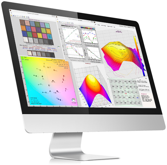
Imatest launches Camera Geometric Calibration Validation Service for ADAS and Autonomous Vehicle companies

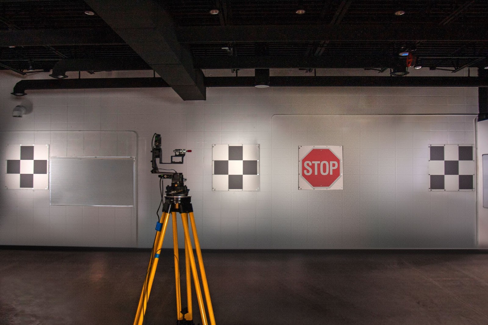
Imatest, LLC, a leader in image quality evaluation tools, today announced the launch of their new Camera Geometric Calibration Validation service to provide objective metrics for calibration quality. The Service uses upcoming IEEE P2020 geometric calibration standard as a reference. (more…)

Read More

Imatest sells exclusive license for intrinsic geometric calibration software to Furonteer

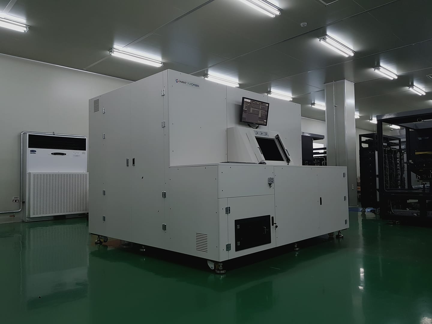
Imatest, LLC, a leader in image quality testing software, analysis, test charts, and test lab equipment, and Furonteer, the forerunner in the field of ADAS/Autonomous Sensing Camera Assembly & Test Equipment, announced that Furonteer has purchased the exclusive license to Imatest’s intrinsic geometric calibration software. The two companies partnered originally in 2019 to launch the Imatest-Furonteer geometric calibration solution. 

(more…)

Read More

Imatest Releases Version 2021.1

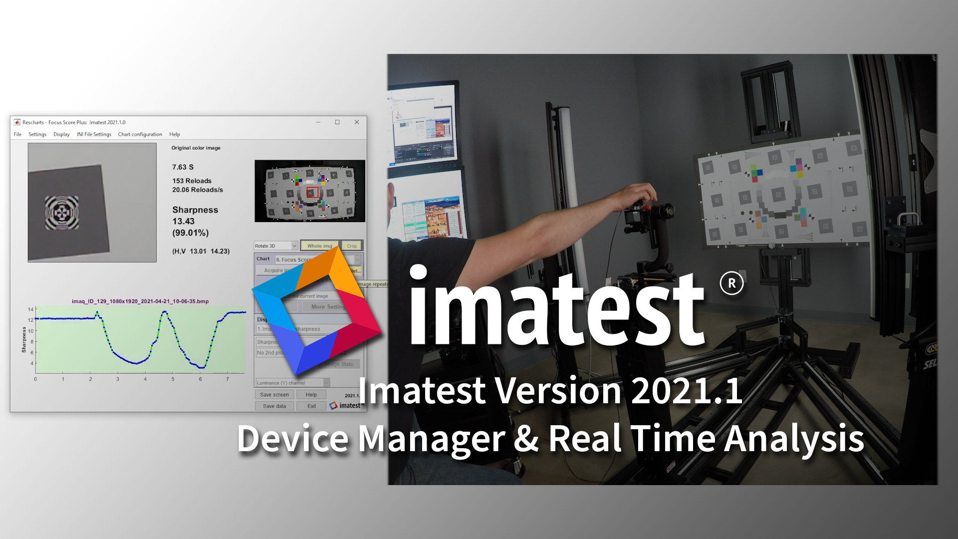
Imatest Version 2021.1 adds several new features to Imatest Master and Imatest IT, including edge tracking during live focusing, alignment tools in device manager, new subjective exposure quality loss calculation, OpenEXR support, live exposure and white balance measurements and several customer-requested features.
(more…)

Read More

Calculating Exposure Quality Loss per IEEE CPIQ v2

CPIQ Auto exposure is in draft status. It will be added to the 2021 revision of the CPIQ Standard. You should use Imatest v2021.1 or later to perform this calculation.

Auto exposure error is based on deviation from a nominal luminance value for the neutral grey patch in an X-Rite Colorchecker SG. In a variant calculation, we can also calculate this metric from a 24-patch X-Rite Colorchecker.

A psychophysical study of the subjective quality based on luminance level was how the following model for exposure quality loss was developed:

CPIQ Auto exposure is measured with the Imatest Color/Tone module, which produces a Quality Loss (QL) score in units of Just Noticeable Differences (JND).

Results are available in display #4 2D a*b:

and display #7 B&W density & White Balance:


For more about Imatest’s CPIQ support click here

Read More

Introducing MTS-RM-NIR

The Imatest MTS Reflective Module integrates with our Modular Test Stand Base Module and one or both of the following lights:

This fixture provides the basic setup for a test lab to perform image quality tests with reflective lighting.

  • Easily and reliably illuminate reflective test charts for efficient testing and robust measurements.
  • High-quality hardware allows you to effortlessly position the LED lights
  • Angle and position markers help you record light bank locations for future testing. 


The Base Module, Target, KinoFlo or Metaphase Lights are sold separately from the Reflective Module.

Read More

Three optical centers

Customers frequently want to know how we measure the optical center of the image (not to be confused with the geometrical center).  They may be surprised that we measure three, shown below in the 2D contour map, which is one of the options in Rescharts slanted-edge modules 3D & contour plots. 

SFRplus contour plot for MTF50P, showing three optical centers:

For a normal well-constructed lens, the optical centers are all close to the geometric center of the image. They can diverge for defective or poorly-constructed lenses.

Center of MTF (Center of Sharpness)

The center of MTF (or Sharpness) is the approximate location of maximum MTF, based on a second-order fit to results for slanted-edge charts (SFRplus, eSFR ISO, Checkerboard, and SFRreg). It is displayed (along with the two other optical centers) displayed in the 2D image contour map, which is one of the options in 3D & Contour plots

Algorithm:  Starting with an array of all MTF50 values and arrays for the x and y-locations of each value (the center of the regions), fit the MTF50 value to a second-order curve (a parabola). For the x (horizontal) direction,

MTF = axx2 + bxx + cx .

The peak location for this parabola, i.e., the

x-Center of MTF = xpeak = –bx /(2ax) .

It is reported if it’s inside the image. (It is not uncommon for it to be outside the image for tilted or defective lenses.) The y-center is calculated in exactly the same way.

MTF asymmetry is calculated from the same data and parabola fits as the Center of MTF. For the x- direction, 

MTF50 (x-aysmmetry) = (MTFfit(R) − MTFfit(L)) / (MTFfit(R) + MTFfit(L))

where MTFfit(R) and MTFfit(L) are the parabola fits to MTF at the left and right borders of the image, respectively. MTF50 (y-asymmetry) is calculated with the same method.

Center of illumination

The center of illumination is the brightest location in the image. It is usually not distinct, since brightness typically falls off very slowly from the peak location. It only represents the lens for very even back-illumination (we recommend one of our uniform light sources or an integrating sphere). For front illumination (reflective charts) it represents the complete system, including the lighting.

It is calculated very differently in Uniformity and Uniformity Interactive than it is in the slanted-edge modules.

Algorithm for Uniformity and Uniformity Interactive:  The location of the peak pixel (even if it’s smoothed) is not used because the result would be overly sensitive to noise. Find all points where the luminance channel g(x,y) (typically 0.2125*R + 0.7154*G + 0.0721*B) is above 95% of the maximum value. The x-center of illumination is the centroid of these values. The y-center is similar. This calculation is much more stable and robust than using peak values.

Cx = ∫x g(x)dx / ∫g(x)dx

Algorithm for Rescharts slanted-edge modules:  Starting with Imatest 2020.2, the mean ROI level of each region is calculated and can be plotted in 3D & contour plots

SFRplus contour plot for mean ROI levels, used to calculate
Center of Illumination ()

The calculation is identical to the Center of MTF calculation (above), except that mean ROI level is used instead of MTF50.

Center of distortion

The center of distortion is the point around which Imatest distortion models assume that distortion is radially symmetric. It is calculated in Checkerboard, SFRplus, and Distortion (the older legacy module) when a checkbox for calculating it is checked. It is calculated using nonlinear optimization. If it’s not checked (or the center is not calculated), the geometrical center of the image is assumed to be the center of distortion.

Distortion measurements are described in Distortion: Methods and Modules.

Link

What is the center of the image?  by R.G. Wilson and S. A. Shafer. Fifteen, count ’em fifteen optical centers. Do I hear a bid for sixteen? Going… going…


Read More

Imatest Names a new Vice-Chairman

Imatest names Rémi Lacombe as Vice Chairman of Imatest LLC to guide our success in 2021 and beyond.

Rémi brings a wealth of experience in the imaging field, which will allow Imatest to better serve our partners and customers.


About Remi

Rémi brings extensive experience to the Imatest Vice Chairman role, leveraging more than 20 years of experience in general management, strategic deals, sales and marketing in the camera and software industry. Rémi is also the SVP Sales and Marketing of Sentons an ultrasonic touch company based in San Jose, CA. Before, Rémi guided DigiLens waveguide technologies into automotive HUD and Augmented Reality smart glasses. Prior to DigiLens, Rémi was VP of Sales and Marketing at InVisage Technologies Inc., an image sensor company acquired by Apple. Earlier in his career, Rémi designed DxO Labs’ imaging technologies into many smartphone devices creating and growing a business that was eventually sold to GoPro.

Rémi received his master’s degree in Engineering Management from Stanford University and holds Applied Science and Engineering degrees from Ecole Polytechnique and Ecole Nationale Superieure des Telecommunications, both in Paris, France.

You can connect with Rémi via LinkedIn here.

Read More

Imatest Founder Norman Koren Receives Lifetime Achievement Award

Imatest LLC Chief Technical Officer and Founder Norman Koren was awarded a Lifetime Achievement Award by AutoSens during the latest AutoSense-Detroit.  In a sparkling virtual ceremony, Norman remarked:

“Thank you all for this unexpected honor, which I appreciate all the more because everyone on the short list is outstandingly qualified. My work in imaging is actually my second career, which I started it when I was sixty. It’s been a real honor to help the industry improve the quality of a wide variety of cameras and a pleasure to get to know some amazing people along the way.”

(more…)

Read More