In the 2021 Electronic Imaging conference (held virtually) we presented a paper that introduced the concept of the noise image, based on the understanding that since noise varies over the image surface, noise itself forms an image, and hence can be measured anywhere, not just in flat patches.
You can download the full paper (in the original PDF format) here.
—— or you can read the HTML version below. ——
Using images of noise to estimate image processing behavior for image quality evaluation
Norman L. Koren, Imatest LLC, Boulder, Colorado, USA
Abstract
Noise is an extremely important image quality factor. Camera manufacturers go to great lengths to source sensors and develop algorithms to minimize it. Illustrations of its effects are familiar, but it is not well known that noise itself, which is not constant over an image, can be represented as an image.
Noise varies over images for two reasons. (1) Noise voltage in raw images is predicted to be proportional to a constant plus the square root of the number of photons reaching each pixel. (2) The most commonly applied image processing in consumer cameras, bilateral filtering [1], sharpens regions of the image near contrasty features such as edges and smooths (applies lowpass filtering to reduce noise) the image elsewhere.
Noise is normally measured in flat, uniformly-illuminated patches, where bilateral filter smoothing has its maximum effect, often at the expense of fine detail. Significant insight into the behavior of image processing can be gained by measuring the noise throughout the image, not just in flat patches.
We describe a method for obtaining noise images, then illustrate an important application— observing texture loss— and compare noise images for JPEG and raw-converted images. The method, derived from the EMVA 1288 analysis of flat-field images, requires the acquisition of a large number of identical images. It is somewhat cumbersome when individual image files need to be saved, but it’s fast and convenient when direct image acquisition is available.
Introduction
Noise is typically measured in flat patches of test charts that include grayscale patterns. While this is convenient and useful for calculating Signal-to-Noise Ratio (SNR), it has several shortcomings. In processed images, noise in flat patches can be strongly affected by software noise reduction, leading to erroneous dynamic range measurements. There is no information on what happens to noise in the presence of image features— texture, edges, etc. It is well known that the human eye is much less sensitive to noise in the presence of detail than in smooth areas (this is why bilateral filtering is effective), but what about machine vision?
In a recent paper [2], we addressed the issue of measuring noise in the presence of a signal for the Siemens star pattern, where the ideal sinusoidal image can be inferred from a noisy acquired image using Fourier analysis. Noise is the difference between the actual and ideal image. This allows MTF to be measured in the same location as noise, partially overcoming the effects of bilateral filtering and enabling a camera information capacity calculation.
To overcome the chief limitation of this technique, which only works with the Siemens star, we have developed a general method for measuring noise anywhere in any image based on temporal noise and Photo Response Nonuniformity (PRNU) measurements in the EMVA 1288 standard [3].
Method
To measure noise throughout an image, i.e., to obtain an image of the noise itself, either (a) capture a set of L identical but independent images, saving them in L files, or (b) capture L images by direct acquisition (if available), which can be extremely efficient since only two image arrays need to be saved. L should be at least 32; 128 is even better.
The mean of each individual pixel in the set of L captured images is
\(\displaystyle \mu_s = \frac{1}{L}\sum_{l=0}^{L-1}y[l]\)
(1)
The temporal noise variance (noise power) of each pixel is
\(\displaystyle \sigma_s^2 = \frac{1}{L-1}\sum_{l=0}^{L-1}\left(y[l]-\frac{1}{L}\sum_{l=0}^{L-1}y[l] \right)^2 = \frac{1}{L-1}\sum_{l=0}^{L-1} \left(y[l]-\mu_s \right)^2 \)
(2)
In this form, the σs2 equation is cumbersome to evaluate, but it can be simplified so that μs and σs2 can be rapidly calculated from just two arrays: the sum and sum of squares of pixels in the set of L images.
\(\displaystyle \sigma_s^2 = \frac{1}{L}\sum_{l=0}^{L-1}y^2[l] – \left(\frac{1}{L}\sum_{l=0}^{L-1}y[l] \right)^2 \)
(3)
The key observation about this result is that since μs and σs2 are calculated for each pixel in the image, they form images themselves.
μs is the more familiar of the two: it is the averaged image, whose Signal-to-Noise Ratio (SNR) improves by decibels (dB) for L captures. Signal averaging is recommended for analyzing images of charts that are highly sensitive to noise, especially Dead Leaves/Spilled Coins charts or the Log Frequency contrast chart (which varies spatial frequency horizontally and contrast vertically in order to measure the effects of image processing).
The noise image is derived from temporal noise variance σs2, which is less familiar. We use its square root, RMS noise voltage σs (which is used in SNR calculations) as the noise image because it has lower contrast than σs2, making it better suited for visualization.
Results
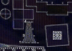
Figures 1 and 2 illustrate the mean μs and RMS temporal noise σs from L = 128 samples for a portion of a modified ISO 12233:2017 chart, acquired by an inexpensive 1920×1080 HD USB camera. “Halos” from strong edge sharpening are visible in Figure 1. As expected, noise (the light bands in Figure 2) is highest near sharp, contrasty features.
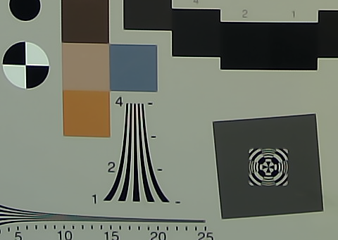
Figure 1. Crop of the averaged the image of modified ISO 12233:2017 chart.
Before we present noise images, we need to explain the challenges and tradeoffs in displaying them.
Noise images displayed with their original scaling (the same as the original image) are usually too dark for visual interpretation. If they are lightened, they make visual sense, but quantitative information (the actual noise levels) is lost. If they are displayed as pseudocolor images, quantitative information is maintained but since a single channel (often a composite channel like the average of R, G, B) must be selected, color information is lost.
Figures 2 and 5 are lightened noise images that contain only qualitative information.
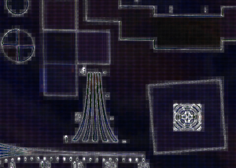
Figure 2. Noise image σs for crop in Fig. 1.
L = 128 acquisitions
Texture measurement quality
Noise images can be used to estimate the reliability of dead leaves (spilled coins) texture blur measurements. In traditional measurements such as the IEEE 1858 Standard for Camera Phone Image Quality,
\(MTF = \sqrt{PSD(image) / PSD(target)}\)
(4)
In older texture calculations, PSD(noise), measured in a flat area near the active pattern, was subtracted from PSD(image) [4], but this technique is being abandoned in recent drafts of the revised standard [5] because of the growing realization that it fails in the presence of bilateral filtering. Signal averaging is now recommended for removing the effects of noise [6].
A key problem with the texture MTF calculation is that it is a bulk measurement that includes both sharpened and lowpass-filtered areas, i.e., it provides no information about spatially-dependent details of texture loss.
Bilateral filters have a threshold that determines the boundary between locally sharpened areas, where MTF is boosted, and locally smoothed areas, where MTF is decreased and fine texture is lost. In Spilled Coins (Dead Leaves) charts, which have a maximum contrast of 3:1, this threshold can be below the maximum pattern contrast, which can make the image processing highly nonuniform. This situation is illustrated by comparing Figure 3, from the inexpensive USB camera, with Figure 4, from a high-quality high-resolution reference camera (similar to the original chart design). In Figure 3, a few contrasty edges are sharp, but most of the fine texture is absent.
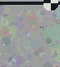 Figure 3. Spilled Coins image crop μs Figure 3. Spilled Coins image crop μs from a 2 megapixel HD USB camera. |
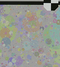 Figure 4. Spilled Coins image crop μs Figure 4. Spilled Coins image crop μs from a high quality reference camera. |
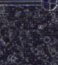
Figure 5. Noise image σsfor Spilled Coins crop
(Figure 3) from a USB camera
In the noise image (Figure 5) corresponding to the USB camera image in Figure 3, light areas have relatively high noise, corresponding to strong sharpening on contrasty edges, and dark areas have relatively low image noise, corresponding to strong lowpass filtering and significant texture loss in low contrast areas, visible by comparing Figures 3 and 4.
The MTF of the averaged image μs (Figure 6) is a misleading indicator of good texture response. It gives little indication of the true behavior of the camera.
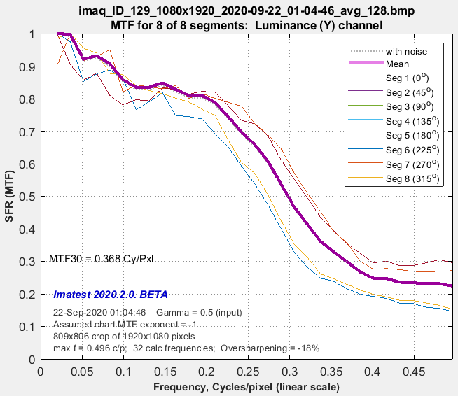
Figure 6. MTF of the averaged image, μs
Raw or minimally-processed images would be expected to have relatively uniform image noise. The uniformity can be quantified by a histogram of the noise image pixel levels.
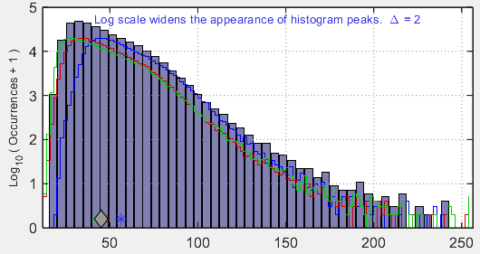
Figure 7. Histogram of noise image (σs)
A narrow histogram would indicate a reliable texture MTF measurement. A wide histogram (as shown in Figure 7) indicates that the MTF is not trustworthy
Comparing raw and JPEG images
We acquired four sets of Spilled Coins images from a high quality mirrorless camera with a 1-inch sensor (the Panasonic Lumix LX-100): JPEG images and raw images converted to TIFF files with minimal processing (using dcraw). Images were acquired at Exposure Index (EI) 200 and 3200 (where low and high noise are expected). Approximately 40 images were acquired for each set.
The JPEG images are highly processed: sharpening and noise reduction have been applied. (The JPEGs are high quality, so JPEG compression artifacts are minimal.)
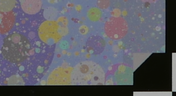
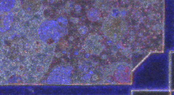
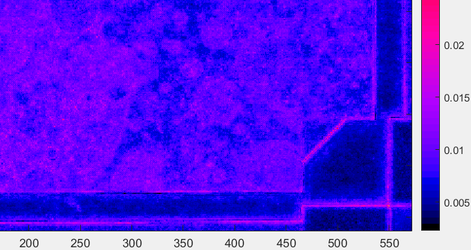
Figure 8. JPEG @ EI 200.
a. (upper) Original image
b. (middle) Lightened (color) noise image
c. (lower) Pseudocolor noise image, showing numeric scale normalized to 1.
A low contrast noise image pattern is visible in the JPEG Spilled Coins area because noise is relatively low at EI 200, so only a small amount of noise reduction was applied. Normalized noise values are in the 0.008-0.014 range. The lightened noise image shows a curious phenomenon: The dominant noise color is the compliment of the dominant image color, e.g., yellowish areas have predominantly blue noise.
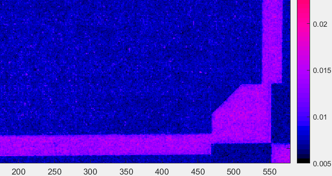
Figure 9. Raw/TIFF @ EI 200. Pseudocolor noise image, showing numeric scale normalized to 1.
Virtually no pattern is visible in the raw/TIFF Spilled Coins area, except for a slight repetitive variation caused by aliasing (not in the actual image). Noise ranges from 0.007-0.009: lower than the JPEG, apparently because the JPEG has significant sharpening but minimal noise reduction.
Note that the black bar below and to the right of the raw/TIFF spilled coins pattern is lighter, i.e., noisier. This is an anomaly that does not fit the expected noise model. We have no good explanation.
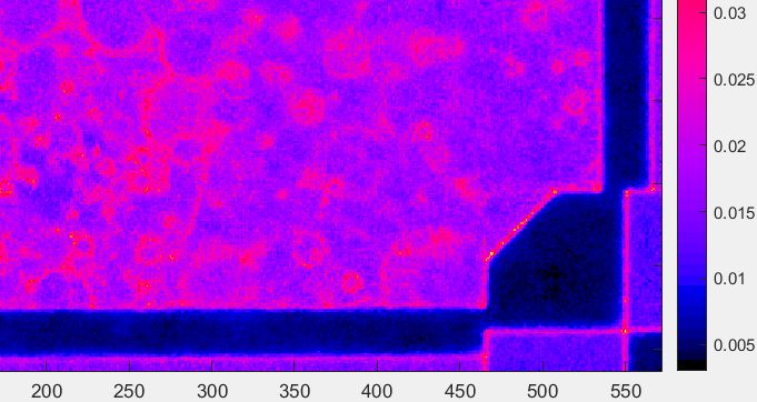
Figure 10. JPEG @ EI 3200. Pseudocolor noise image, showing numeric scale normalized to 1.
A much stronger pattern is visible than for the EI 200 JPEG. Noise values range from 0.012-0.024.
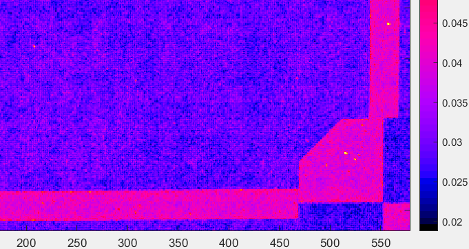
Figure 11. Raw/TIFF @ EI 3200. Pseudocolor noise image, showing numeric scale normalized to 1
Noise values range from 0.028-0.036, higher than for the JPEG, which has had significant noise reduction applied. As with EI 200, the black bar has more noise than expected.
Noisy pixel defect
An interesting observation from the mirrorless camera (which is several years old, so its sensor may not be “as good as new”) is a type of defect pixel that doesn’t reliably show up in hot or dead pixel measurements — noisy pixels.
Such a defect is visible in the JPEG EI 200 pseudocolor image. (It is present in all the noise images, but harder to see.)
Noisy pixels are best measured with flat-field images.
Noisy pixels are generally not clearly visible in averaged images. Since they vary from image to image, they can be difficult to measure from single images. The only reliable way to find them is to acquire a large number of images, which may be impractical in production environments, but can be done with moderate efficiency (in a few seconds) if direct image acquisition is available.
Another type of defect we haven’t studied is the stuck pixel, which is not necessarily light nor dark. A stuck pixel would have zero noise. We haven’t found any in our limited set of images.
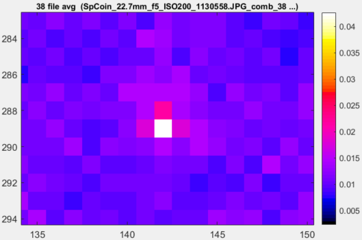 Figure 12. Noisy pixel defect in highly enlarged JPEG @ ISO 200 pseudocolor noise image.
Summary and future work
The technique presented here allows noise to be measured anywhere in an image, not just in flat, uniform areas. Noise itself is treated as an image.
The noise image can be used to examine details of image processing such as the operation of bilateral filters— to view where they sharpen and where they smooth the image. It can potentially reveal sensor and image processing artifacts.
As we indicated earlier, displaying the noise image presents challenges and tradeoffs, largely because noise varies rapidly in the areas of greatest interest— near lines, edges, and other contrasty features. This problem is intrinsic to any result with rapid spatial variation. It is easier to display slowly-varying measurements such as signal or noise in flat test chart patches. But we are interested in information that is missing in flat patches.
We hope to use noise images to develop improved texture loss measurements and perhaps to develop local information capacity measurements for optimizing machine vision image processing.
To summarize, noise images are a potentially valuable tool for analyzing and optimizing imaging systems. We are confident that they will find uses that have yet to be discovered.
References
- Tomasi, C., and R. Manduchi. “Bilateral Filtering for Gray and Color Images”, Proceedings of the 1998 IEEE International Conference on Computer Vision. Bombay, India. Jan 1998, pp. 836–846.
- Koren, “Measuring camera Shannon Information Capacity with a Siemens Star Image”, Electronic Imaging 2019, Society for Imaging Science and Technology.
- European Machine Vision Association, EMVA 1288 standard, emva.org/standards-technology/emva-1288/
- McElvain, S. Campbell, J. Miller, E. Jin, “Texture-based measurement of spatial frequency response using the dead leaves target: extensions, and application to real camera systems”, Electronic Imaging 2010, https://www.imaging.org/site/PDFS/Reporter/Articles/2010_25/Rep25_2_EI2010_MCELVAIN.pdf
- Koren, B. Tseng, Q. Wang, et al., “IEEE p1858 v2 Standard for Camera Phone Image Quality”, https://sagroups.ieee.org/1858/ [Draft Publication Late-2021 – Early-2022]
- Suresh, T. J. Pfefer, J. Su, Y. Chen, and Q. Wang, “Improved texture reproduction assessment of camera-phone-based medical devices with a dead leaves target,” OSA Continuum 2, 1863-1879 (2019).
Author biography
Norman Koren became interested in photography while growing up near the George Eastman House photographic museum in Rochester, NY. He received his BA in physics from Brown University (1965) and his Masters in physics from Wayne State University (1969). He worked in the data storage industry simulating digital magnetic recording systems and channels for disk and tape drives from 1967-2001. In 2003 he founded Imatest LLC to develop software and test charts to measure the quality of digital imaging systems.