|
News: Imatest 23.1 (March 2023) (available in the Imatest Pilot program). New methods for calculating Camera information capacity, Noise Power Spectrum (NPS), Noise Equivalent Quanta (NEQ), Ideal observer SNR (SNRi), and Noise autocorrelation from slanted-edge patterns are now available. |
|
The basic premise of this work is that Information capacity is a superior The revised 2020 white paper, “Camera information capacity from Siemens Stars“, briefly introduces information theory, describes the Siemens star camera information capacity measurement, then shows results (including the effects of artifacts). A more recent white paper (2023), “Measuring Information Capacity with Imatest“, describes a method of measuring information capacity and related measurements (NPS, NEQ, SNRi, and more) from widely-used slanted edges.
|
Introduction – Summary diagram – Edge variance calculation – Noise method 1 – Noise method 2
Noise image calculation – NPS – NEQ – SNRi – CSNRi – Object visibility – Noise Autocorrelation
Meaning of Information capacity – Summary – Links – Binning noise – Calculating Cmax
Instructions page: Acquiring and framing – Running the MTF module – Results – Edge/MTF plot
Edge/noise plot – 3D plot and Total information capacity –
Claude Shannon
Nothing like a challenge! There is such a metric for electronic communication channels— one that quantifies the maximum amount of information that can be transmitted through a channel without error. The metric includes sharpness and noise (grain in film). And a camera— or any digital imaging system— is such a channel.
The metric, first published in 1948 by Claude Shannon* of Bell Labs [1,2], has become the basis of the electronic communication industry. It’s called the Shannon channel capacity or Shannon information capacity C, and has a deceptively simple equation [3]. (See the Wikipedia page on the Shannon-Hartley theorem for more detail.)
\(\displaystyle C = W \log_2 \left(1+\frac{S}{N}\right) = W \log_2 \left(\frac{S+N}{N}\right) = \int_0^W \log_2 \left( 1 + \frac{S(f)}{N(f)} \right) df\)
W is the channel bandwidth, S(f) is the average signal energy (the square of signal voltage; proportional to MTF(f)2), and N(f) is the average noise energy (the square of the RMS noise voltage), which corresponds to grain in film. It looks simple enough (only a little more complex than E = mc2 ), but it’s not easy to apply.
*Claude Shannon was a genuine genius. The article, 10,000 Hours With Claude Shannon: How A Genius Thinks, Works, and Lives, is a great read. There are also a nice articles in The New Yorker and Scientific American. And IEEE has an article connecting Shannon with the development of Machine Learning and AI. The 29-minute video “Claude Shannon – Father of the Information Age” is of particular interest to me it was produced by the UCSD Center for Memory and Recording Research. which I frequently visited in my previous career.
This page describes how to calculate information capacity C from images of slanted-edges, Imatest’s most widely-used test image, which (thanks to a recent discovery) allows signal and noise to be calculated from the same location, resulting in a superior measurement of image quality. The earlier (2020) Siemens star method is described in Shannon information capacity from Siemens stars.
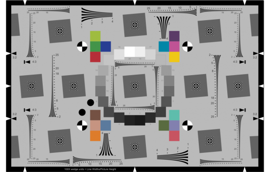
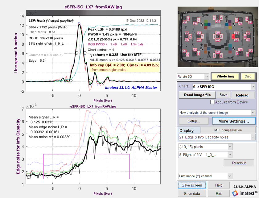
The eSFR ISO chart. Automatically detected ROIs, combining MTF, color, tone, and noise measurements
Introduction to the new measurements
This page describes several Information capacity-related measurements introduced in Imatest 23.1, released in March 2023. These measurements take advantage of newly-discovered properties of slanted edges– Imatest’s most widely used patterns for measuring MTF. Many have been used for medical imaging, but are unfamiliar elsewhere, in part because they were difficult to perform. We describe two convenient new measurement methodologies, both of which use the slanted edge.
- The Edge variance calculation conveniently calculates camera information capacity.
- The Noise image calculation, which uses a different approach to calculate information capacity and several additional image quality factors (Noise Power Spectrum (NPS), Noise Equivalent Quanta (NEQ), SNRi, Noise autocorrelation, and more).
|
This page introduces the new calculations and presents detailed equations and algorithms. The Instructions page introduces the new calculations, shows how to obtain them, then presents Key Results. |
Motivation — We need to obtain information capacity from images that have very different types of image processing.
- Minimally or uniformly-processed images, converted from raw to TIFF or PNG files. By “minimally-processed”, we mean no sharpening, no noise reduction, at most a simple gamma curve (no complex tonal response curves or local tone mapping). A color matrix may be applied (it affects noise and SNR, but not MTF). When available, these images give the most reliable information capacity measurements.
- JPEG files from cameras, which usually have bilateral filters — filters that sharpen images near contrasty features like edges but blur them to reduce noise elsewhere — making it appear that the image contains more information than it actually has. This improves conventional SNR measurements (made from flat patches) while actually removing information.
In late October 2022, we discovered how to extract signal-dependent noise from slanted-edges using an overlooked capability of the ISO 12233 slanted-edge algorithm, described briefly below and in more detail in the white paper, Measuring Camera Information Capacity from Slanted-edges.
In March 2023, we discovered a second overlooked capability that allows Imatest to calculate a camera’s Noise Power Spectrum (NPS), Noise Equivalent Quanta (NEQ), and Ideal Observer SNR (SNRi), but only works with minimally / uniformly-processed images.
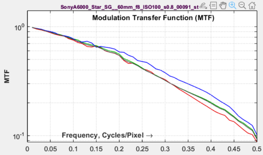
The slanted-edge method of calculating MTF, which has been part of the ISO 12233 standard since 2000,
- takes each scan line yl (x) in a slanted-edge Region of Interest (ROI),
- finds its center,
- fits a polynomial curve to the centers, then
- depending on the relation between the line center and the curve, adds the line contents to one of four bins.
- The bins are then interleaved, resulting in a 4× oversampled averaged edge, which has lower noise than the individual scan lines.
- Calculates MTF (Modulation Transfer Function, usually synonymous with Spatial Frequency Response), by differentiating the averaged edge to obtain the Line Spread Function, LSF, windowing the LSF, then Fourier-transforming it. MTF is the absolute value of the Fourier Transform normalized to 1 (or 100%) at zero frequency.
The new information capacity measurements take advantage of overlooked capabilities of the slanted-edge method.
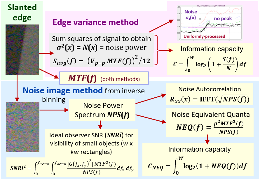 Summary diagram: Both methods use MTF(f) in information capacity calculations.
The Noise image method requires uniformly-processed images.
It calculates NPS, NEQ, and SNRi, and Rxx in addition to C.
A: Edge variance calculation
Summary: Sum the squares of the scan lines to obtain the edge variance, then use it to calculate information capacity.
The Edge variance Information capacity calculation is described in detail in the white paper, New Slanted-Edge Image Quality Measurements: the Edge variance calculation, and in the paper presented at Electronic Imaging 2023, “Measuring Camera Information Capacity with Slanted Edges“.
The calculation starts with images of slanted edges, (Original ROI, below), typically made from a 4:1 contrast chart (chart contrasts between 2:1 and 10:1 are acceptable). In addition to the binning/summing described above, the squares of the scan lines are summed. This allows the variance of the edge, σs2(x), which is equivalent to the signal-dependent noise power, N(x), to be calculated.
\(\displaystyle \sigma_s^2(x) = \frac{1}{L} \sum_{l=0}^{L-1} (y_l(x)-\mu_s(x))^2 = \frac{1}{L}\sum_{l=0}^{L-1} y_l^2(x) \ – \left(\frac{1}{L}\sum_{L=0}^{L-1} y_l(x) \right)^2 \)
Noise power for the Shannon-Hartley Equation N(x) = σs2(x) and voltage σs(x) are important because many images— including most JPEGs from consumer cameras— have bilateral filters, which sharpen the image (boosting noise) near sharp areas like edges, and blurs it (to reduce visible noise) elsewhere. This obscures the noise at edges, which is critical to the performance — and information capacity — of the system. The new technique makes signal-dependent noise near the edge visible so that it can be used in the information capacity calculation. It is also highly convenient.
The selection of N depends on the image processing. Two major classes have been identified.
- Uniformly or minimally-processed images, often TIFFs converted from raw files (raw→TIFF) without bilateral filtering, i.e., they either have no or uniform sharpening or noise reduction. Most cameras intended for Machine Vision/Artificial Intelligence fall into this category.
Since noise can be a very rough function of x, a large region size is required for a stable value of N. We average over all values of x in the ROI.
\(N_{uniform} = \text{mean}(\sigma_s^2(x))\) for all values of x in the ROI. - Bilateral-filtered images include most JPEG images from consumer cameras.
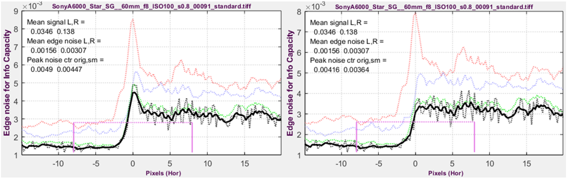
Bilateral filters sharpen images near contrasty features such as edges, but blur them (to reduce noise) elsewhere. This causes a noise peak near the edge (below, left). The blurring improves Signal-to-Noise Ratio (SNR), but it removes information. Because of this, noise near the edge can dominate camera performance, and should be strongly weighted in calculating N. We have long known about the noise peak, but until the present method was developed, there was no easy way to observe or measure it (or detect bilateral filtering).
For calculating information capacity C, we use the square of the voltage, σ, at the peak, smoothed (with a rectangular kernel of length PW20/2) to remove jaggedness. \(N_{bilateral} = \sigma^2_{peak}\). This is a somewhat arbitrary choice that produces reasonably consistent results. This method also works with uniformly-processed images, but results are less consistent.
Imatest lets you select the calculation of noise N: it can be Nuniform, Nbilateral , or automatically detected depending on the presence of a peak.
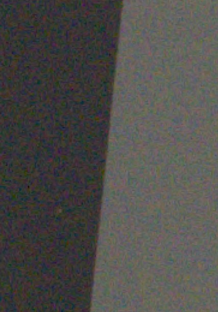
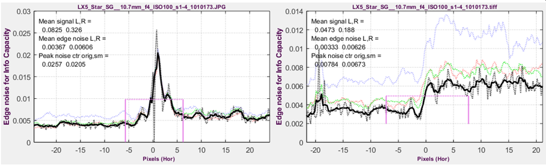 Edge noise voltage for compact camera @ ISO 100. Left: Bilateral-filtered in-camera JPEG; Right Unsharpened TIFF from raw.
The x-axis is the original pixel location of the 4× oversampled signal.
Voltage statistics for the slanted edge
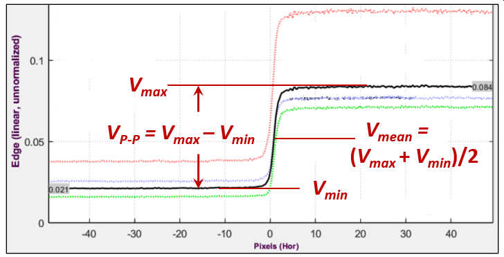
Signal power S for the Shannon-Hartley Equation The mean signal amplitude for a uniformly-distributed signal of peak-to-peak amplitude VP-P is \(V_{avg}(f) = V_{P-P} MTF(f) / \sqrt{12}\) — a reasonable number to use for the information capacity calculation using the Shannon-Hartley equation, shown above, which actually uses the average signal power, \(S_{avg}(f) = V^2_{P-P} MTF(f)^2 / 12\).
After removing newly-discovered binning noise, selecting noise power calculation, and adjusting the signal level from the edge, which is a square wave, to be more representative of an “average’ signal, numbers are entered into the Shannon-Hartley equation (above) to calculate the information capacity, for the chart contrast.
Bandwidth W is always 0.5 cycles/pixel (the Nyquist frequency). Signals above Nyquist do not contribute to the information content; they can reduce it by causing aliasing — spurious low frequency signals like Moiré that can interfere with the true image. Frequency-dependence comes from MTF(f).
Savg(f), N, and W are entered into the Shannon-Hartley equation to obtain information capacity C.
\(\displaystyle C = \int^{0.5}_0{\log_2\left(1+\frac{S_{avg}(f)}{N}\right)}df \ \approx \sum_{i=0}^{0.5/\Delta f} {\log_2\left(1+\frac{S_{avg}(i\Delta f)}{N}\right)} \Delta f \)
The key results are
C4 is the direct result of measuring 4:1 contrast ratio slanted-edges. It is calculated from the Shannon Hartley equation, using several assumptions (that the signal is uniformly distributed over the peak-to-peak measurement and the noise power spectral density (NPD) is flat). C4 is a special case of Cn, for a n:1 contrast ratio (with ISO standard 4:1 strongly recommended) Cn is sensitive to chart contrast ratio and exposure, making it interesting for measuring performance as a function of exposure but less robust than ideal for calculating a camera’s maximum information capacity.
Cmax (derived in Appendix 2) is a much more stable measurement of the maximum information capacity for the camera starting with C4 (for the 4:1 contrast chart). It is also insensitive to exposure, at least for linear sensors, where noise is a known function of signal voltage.
Here are some key results of the Edge variance method.
 Line Spread Function (LSF) and signal-dependent noise σ from
eSFR ISO image converted from raw with minimal processing
B. Noise image calculation
Summary: Subtract a low-noise reverse-projected / de-binned ROI image from the original image to obtain a noise image, which can be used to calculate Noise Power Spectrum (NPS) and several additional measurements.
| Measurement | Description |
| Noise Power Spectrum, NPS(f) | NPS was implicitly assumed to be constant (white noise) in the Edge variance method. |
| Noise Equivalent Quanta, NEQ(f) and NEQinfo(f) |
measures of frequency-dependent signal-to-noise ratio (SNR). \(NEQ(f) = \mu^2\ MTF^2(f) / NPS(f)\text{, where }\mu = V_{mean}\) has been used for quantifying medical image quality, but are much less familiar in general imaging. NEQ(f) is equivalent to the number of quanta detected by the sensor when photon shot noise is dominant. It is appropriate for calculating Digital Quantum Efficiency (DQE), when the density of quanta reaching the image sensor is known. NEQinfo(f) is derived from \(\mu = V_{P-P} / \sqrt{12}\), making it well-suited for calculating information capacity CNEQ. |
| Information capacities C4-NEQ and Cmax-NEQ |
correspond to C4 and Cmax (Appendix 2) from the Edge variance method, but are derived from NEQinfo(f). They are close, but not identical. |
| Ideal observer Signal-to-Noise Ratio, SNRi | From Skorka and Kane [9], “The Ideal Observer is a Bayesian decision maker that maximizes the statistical precision of a hypothesis test with two possible outcomes.” SNRi as we present is, is a metric of the detectability of small objects (squares or rectangles), typically of low contrast. |
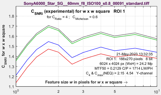
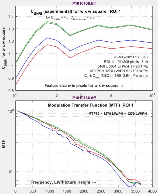
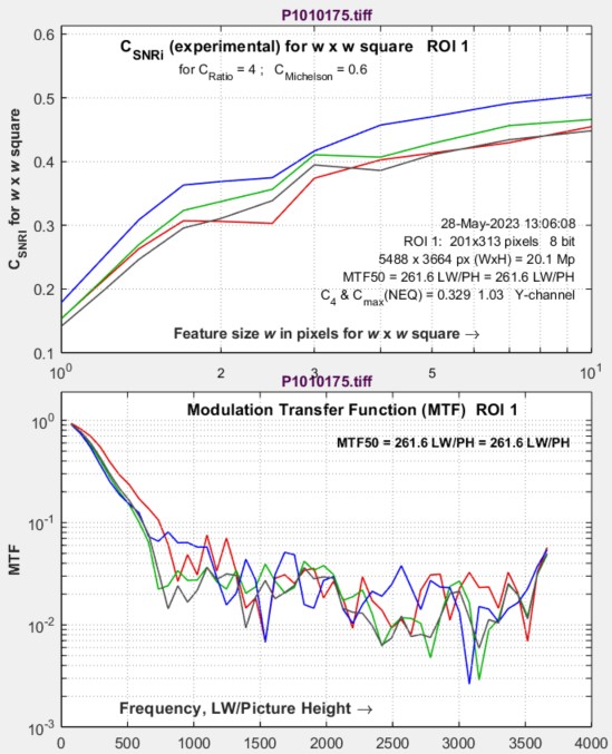
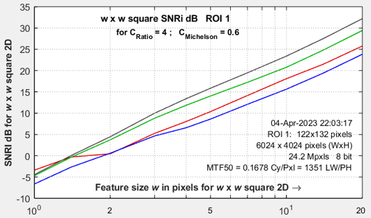
| SNRi information capacity CSNRi (experimental) | CSNRi is a new and experimental measurement (we’re working to verify it) of SNRi-based information capacity, which is plotted as a function of (square or rectangle) side width w. |
| Noise autocorrelation | The inverse Fourier transform of the Noise Voltage Spectrum. Related to sensor electrical crosstalk. |
| Instructions for plotting these results are on the Information Capacity… Instructions page. |
The Noise Image method is the second of two methods for calculating information capacity and related figures of merit. It was developed shortly after the Edge Variance method. It offers a particularly rich set of measurements.
This method involves inverting the ISO 12233 binning procedure. Noting that the 4× oversampled edge was created by interleaving the contents of 4 bins, each of which contains an averaged (noise-reduced) signal derived from the original image, we apply an inverse of the binning algorithm to set the contents of each scan line to its corresponding interleave (Inverse binned… ROI, below). Since the inverse-binned image is a nearly noiseless replica of the original image, we can create a noise image by subtracting the inverse-binned image from the original image. This image is shown, adjusted to make the mean (zero) value middle gray, as the Noise image ROI, on the right below.
A noise image can be created by subtracting the reverse-projected image from the original image, correct for nonuniformity along the direction of the edge. The three images are shown below. The noise image (below-right), which has a mean value of 0, has been lightened and contrast-boosted for display. The three images are linear: a gamma curve has been applied for display.
 Original ROI Original ROI |
 Inverse-binned / de-interleaved / Inverse-binned / de-interleaved /reverse-projected ROI |
 Noise image ROI Noise image ROI |
These images allow several key image quality parameters to be calculated, including Noise Power Spectrum and Noise Equivalent Quanta, well-known in medical imaging systems, and described in an excellent review paper by Ian Cunningham and Rodney Shaw [4]. These measurements are not well-known outside of medical imaging, largely because they have been difficult to measure.
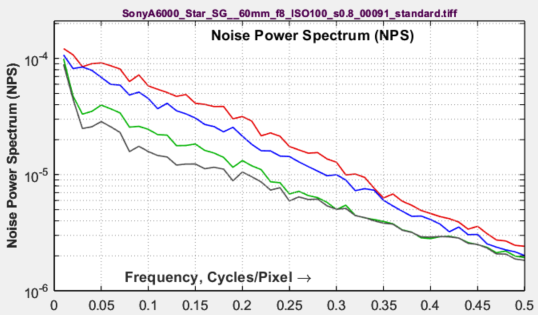 Noise Power Spectrum (NPS)
(the square of the Noise (voltage) spectrum) is calculated by taking the 2D Fourier transform of the noise ROI (Region of Interest) and noting that the initial 2D spectrum has zero frequency at the center of the image. A 1D Noise Power Spectrum, NPS1, is calculated by dividing the 2D spectrum into several annular regions (the number depends on the size of the ROI), then taking the average noise power of each region. This transformation allows calculations to be performed in one dimension (rather than two) under the assumption that the vertical and horizontal MTFs are close.
The relationship between NPS and the variance of the noise image is given in equations (3) and (8) of Cunningham and Shaw [4], which we have reduced to one dimension and with the integration limits changed from {-∞,∞} to {0, fNyq}, where fNyq = Nyquist frequency = 0.5 cycles/pixel.
\(\displaystyle \sigma^2 = \int_0^{f_{Nyq}} NPS(f) df \)
The 1D Fourier transform described above must be scaled to be consistent with the above equation.
\(\displaystyle NPS(f) = \frac{NPS_1(f)\ \sigma^2}{\displaystyle \int_0^{f_{Nyq}} NPS_1(f) df }\)
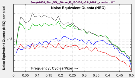 Noise Equivalent Quanta (NEQ)
is a well-known figure of merit in medical imaging, but is unfamiliar in general imaging. It is described in a 2016 paper by Brian Keelan [5]. Essentially, it is a frequency-dependent Signal-to-Noise (power) Ratio. Units are the equivalent number of quanta that would generate the measured SNR when photon shot noise is dominant.
\(\displaystyle NEQ(f) = \frac{\mu^2 MTF^2(f)}{NPS(f)}\)
where the mean linear signal, μ, can be defined in either of two ways, depending on how NEQ is to be interpreted.
If NEQ is to be used for calculating DQE (Digital Quantum Efficiency), where \(DQE(f) = NEQ(f) / \overline{q}\), then μ should be the mean value of the linearized signal voltage in the original image. Measuring DQE requires a separate measurement of the mean number of quanta reaching each pixel. We may add this in the future.
Getting familiar with the meaning and use of NEQ will take some time. Characterization of imaging performance in differential phase contrast CT compared with the conventional CT: Spectrum of noise equivalent quanta NEQ(k) by Tang et. al. is an excellent example of how NEQ is used in medical imaging: it has real technical depth.
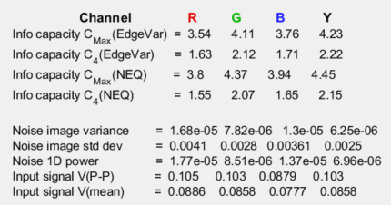 Information capacity from NEQ:
A special form of NEQ, NEQinfo(f), calculated using \(\mu = V_{P-P}/\sqrt{12}\), is used to calculate information capacity, CNEQ, from a special case of the Shannon-Hartley equation. NEQinfo is not plotted.
\(\displaystyle C_{NEQ} = \int_0^W \log_2 \left( 1 + NEQ_{info}(f)\right) df\)
where bandwidth W is the camera’s Nyquist frequency, \(W = f_{Nyq} = 0.5 \text{ Cycles/Pixel}\). [Author’s note: I thought I’d discovered this connection, but it’s in papers on PET scanners and Digital Mammography by Christos Michail et. al. [6,7] Not papers anybody outside medical imaging is like to chance upon.]
Ideal Observer SNR (SNRi)
is a measure of the detectability of small objects. It is described in papers by Paul Kane [8] and Orit Skorka and Paul Kane [9].
[8] presents the SNRi equation in one dimension, but after considerable effort, we determined that the two-dimensional equation in [9] gives the correct results.
\(\displaystyle SNRi^2 = \int \int \left( \frac{\mu^2 \Delta S^2(\nu_x,\nu_y) MTF^2(\nu_x,\nu_y) }{NPS(\nu_x,\nu_y)} \right) d\nu_xd\nu_y \)
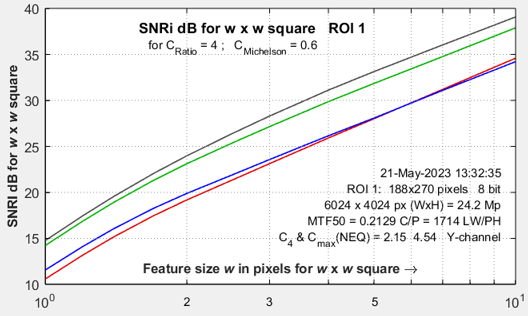
SNRI curves, Micro 4/3 camera, ISO 100
G(νx,νy)2 is the same as μ2ΔS2(νx,νy). MTF(ν) and NPS(ν) are defined in one dimension, where spatial frequency \(\nu = \sqrt{\nu_x^2+\nu_y^2}\) has units of Cycles/Pixel, and the linearized signal is normalized to a maximum value of 1.
The object to be detected is typically a rectangle of dimensions w × kw, where k = 1 (for a square) or 4 for a 1×4 aspect ratio rectangle. Its amplitude (for the initial analysis) is the peak-to-peak voltage of the slanted edge (shown in the Voltage statistics figure, above), \(\Delta Q = V_{P-P}\) which is typically obtained from a chart with a 4:1 contrast ratio.
\(\displaystyle \Delta g(x,y) = \Delta Q \cdot \text{rect}(x/w) \cdot \text{rect}(y/kw)\) ,
where rect(x) = 1 for -1/2 < x < 1/2 ; 0 otherwise.
G(νx,νy) is the Fourier transform of the object to be detected, Δg(x,y). It is expressed in two dimensions.
\(\displaystyle G(\nu_x,\nu_y) = kw^2 \Delta Q \frac{\sin(\pi w \nu_x)}{\pi w \nu_x} \ \frac{\sin(\pi kw \nu_y)}{\pi k w \nu_y} \)
SNRI2 is calculated numerically by creating a two dimensional array of frequencies (0 to 0.5 c/p in 51 steps) that has νx on the x-axis νy on the y-axis, and is filled with \(\nu = \sqrt{\nu_x^2+\nu_y^2}\). These frequencies are used to create a 2D array that can be numerically summed [9].
\(\displaystyle SNRi^2 = \Delta \nu_x \Delta \nu_y \sum_{i=1}^{N_x} \sum_{j=1}^{N_y} \frac{MTF^2(i,j)\ V_{P-P}^2}{NPS(i,j)} \Delta S^2(i,j) \)
SNRi is displayed for each color channel for widths w from 1 to 10. The latest values, which emphasize smaller objects, are w = 1, 1.2, 1.4, 1.7, 2, 2.5, 3, 4, 7, 10. Objects of widths >10 were formerly analyzed, but they provide little insight into system performance.
Object visibility
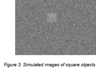 The goal of SNRi measurements is to predict object visibility for small, low contrast squares or 4:1 rectangles The SNRi prediction begs for visual confirmation. A simulated image that can do this is shown in Figure 3 of a classic SNRi paper [8].
We have developed a display for Imatest that does this with a real slanted-edge image and a bit of smoke and mirrors. Despite the trickery, the data is directly from the acquired image.
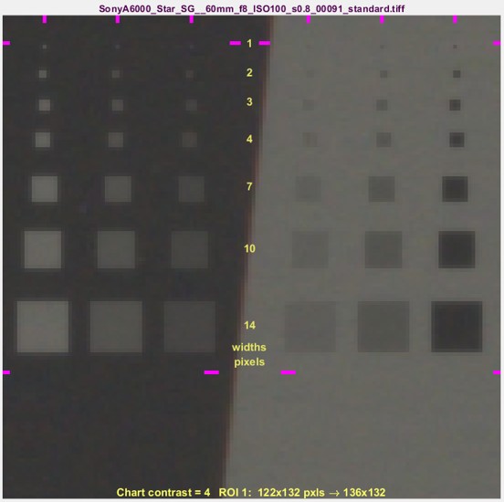
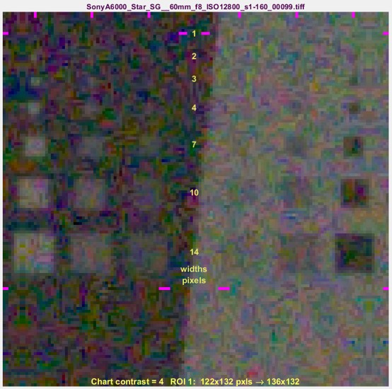
We show two sets of results: one for a relatively low noise image and one high noise image (both from a camera with Micro Four-Thirds sensors, at ISO 100 and 12800, respectively. The sides of the squares are w = 1, 2, 3, 4, 7, 10, 14, and 20 pixels. The original chart has a 4:1 contrast ratio (light/dark = 4), equivalent to a Michelson contrast CMich ((light-dark)/(light+dark)) of 0.6. The outer squares have CMich = 0.6. The middle and inner squares have CMich = 0.3 and 0.15, respectively.
How to use these images — Inconspicuous magenta bars near the margins are designed to help finding the small squares, which are hard to see. The yellow numbers are the square widths in pixels. The SNRi curves (initially, at least) represent the chart contrast — with 4:1 (the ISO 12233 standard) strongly recommended. The outer patches correspond to the SNRi curves, where, according to the Rose model [4], SNRi of 5 (14 dB) should correspond to the threshold of visibility.
|
Low noise image, ISO 100 |
Noisy image, ISO 12800 |
 SNRI curves, Micro 4/3 camera, ISO 12800 Only original pixels were used in these two images, but we used a little smoke and mirrors to make the squares with borders that have the same blur as the device under test. The SNRi curve on the right is for the noisy ISO 12800 image on the right, above. The w = 1 squares are invisible; the w = 2 and 3 squares are marginally visible, and w = 4 squares are clearly visible. In the plot, SNRi at w = 2 is 0-5 dB; it’s 5-10 dB for w =3; close to the expectation that the threshold of visibility is around 14 dB. How the squares were made
|
|
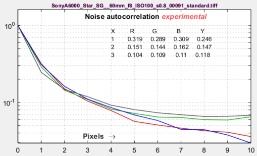
Noise autocorrelationThis plot, which is still in the R&D phase, has been added to examine the hypothesis that the noise power spectrum (and autocorrelation) indicate the amount of electrical crosstalk of image sensor when the effects of demosaicing and fixed-pattern noise are removed and the primary noise source is photon shot noise. The idea behind the hypothesis is that light incident on the sensor is entirely uncorrelated, so that if there were no crosstalk the noise would be white. This image on the right was white-balanced. The curve is the |inverse Fourier transform| of the noise spectrum, based on the author’s limited understanding of the Wiener-Khinchin theorem. |
 |
|
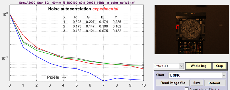
The image on the right is not White-Balanced. The red channel has a larger autocorrelation distance than the other channels, as we would expect. Click on the image to enlarge it. A similar autocorrelation plot can also be obtained from a flat field image in the Image Statics module. Illumination nonuniformity has been corrected to decrease the (spurious) autocorrelation at large distances. |
 |
|
|
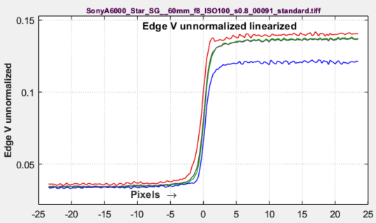
Edge voltage unnormalized — used in the NEQ calculation. |
Meaning of Shannon information capacity
(The Appendix in the white paper, Measuring Information Capacity with Imatest,
has a concise definition of information.)
In electronic communication channels the information capacity is the maximum amount of information that can pass through a channel without error, i.e., it is a measure of channel “goodness.” The actual amount of information depends on the code— how information is represented. But although coding is integral to data compression (how an image is stored in a file), it is not relevant to digital cameras. What is important is the following hypothesis:
Hypothesis: Perceived image quality (assuming a well-tuned image processing pipeline) and also the performance of machine vision and Artificial Intelligence (AI) systems, is proportional to a camera’s information capacity, which is a function of MTF (sharpness), noise, and artifacts arising from demosaicing, clipping (if present), and data compression.
I stress that this statement is a hypothesis— a fancy mathematical term for a conjecture. It agrees with my experience and with numerous measurements, but it needs more testing and verification. Now that information capacity can be conveniently calculated with Imatest, we have an opportunity to learn more about it.
The information capacity, as we mentioned, is a function of both bandwidth W and signal-to-noise ratio, S/N.
|
In texts that introduce the Shannon capacity, bandwidth W is often assumed to be the half-power frequency, which is closely related to MTF50. Strictly speaking, W log2(1+S/N) is only correct for white noise (which has a flat spectrum) and a simple low pass filter (LPF). But digital cameras have varying amounts of sharpening, which can result in response curves with response that deviate substantially from simple LPF response. For this reason we use the integral form of the Shannon-Hartley equation: \(\displaystyle C = \int_0^W \log_2 \left( 1 + \frac{S(f)}{N(f)} \right) df = \int_0^W \log_2 \left(\frac{S(f)+N(f)}{N(f)} \right) df \) S and N are mean values of signal and noise power; they are not directly tied to the camera’s dynamic range (the maximum available signal). For this reason, we reference calculations of C to the contrast ratio of the chart used for the measurement, most frequently C4 for 4:1 contrast charts that conform to the ISO 12233 standard. For Siemens star analysis, we this equation was altered to account for the two-dimensional nature of pixels by converting it to a double integral, then to polar form, than back to one dimension. But this wasn’t necessary for slanted-edges, which are already one dimensional. |
The beauty of both the Siemens Star and Slanted-edge methods is that signal power S and noise power N are calculated from the same location: important because noise is not generally constant over the image.
Summary
- Shannon information capacity C has long been used as a measure of the goodness of electronic communication channels. It specifies the maximum rate at which data can be transmitted without error if an appropriate code is used (it took nearly a half-century to find codes that approached the Shannon capacity). Coding is not an issue with imaging. Rodney Shaw’s paper from 1962 [10] is a particularly good example of measuring C for photographic film— it wasn’t easy back then.
- C is ordinarily measured in bits per pixel. The total capacity is \( C_{total} = C \times \text{number of pixels}\).
- The channel must be linearized before C is calculated, i.e., an appropriate gamma correction (signal = pixel level gamma, where gamma ≅ 2.2 for images in standard color spaces such as sRGB or Adobe RGB) must be applied to obtain correct values of S and N. The value of gamma (close to 2) can be determined from runs of any of the Imatest modules that analyze grayscale step charts: Stepchart, Colorcheck., Color/Tone, Multitest, SFRplus, or eSFR ISO. But in most cases it can be determined from the edge image if the chart contrast is entered and Use for MTF is checked.
- We hypothesize that C can be used as a figure of merit for evaluating camera quality, especially for machine vision and Artificial Intelligence cameras. (It doesn’t directly translate to consumer camera appearance because they have to be carefully tuned to reach their potential, i.e., to make pleasing images). It provides a fair basis for comparing cameras, especially when used with images converted from raw with minimal processing.
- Imatest calculates the Shannon capacity C for the Y (luminance; 0.212*R + 0.716*G + 0.072*B) channel of digital images, which approximates the eye’s sensitivity. It also calculates C for the individual R, G, and B channels as well as the Cb and Cr chroma channels (from YCbCr).
- Shannon capacity has not been used to characterize photographic images because it was difficult to calculate and interpret. But now it can be calculated easily, its relationship to photographic image quality is open for study.
- Since C is a new measurement, we are interested in working with companies or academic institutions who can verify its suitability for Artificial Intelligence systems.
|
Note: A slanted-edge information capacity measurement used prior to Imatest 2020, used primarily to obtain total information capacity from Siemens star measurements, has been deprecated completely because it was not sufficiently accurate. |
Links (more links in the White Paper)
- C. E. Shannon, “A mathematical theory of communication,” Bell Syst. Tech. J., vol. 27, pp. 379–423, July 1948; vol. 27, pp.
623–656, Oct. 1948. - C. E. Shannon, “Communication in the Presence of Noise”, Proceedings of the I.R.E., January 1949, pp. 10-21.
- Wikipedia – Shannon Hartley theorem has a frequency dependent integral form of Shannon’s equation that is applied to both Imatest’s sine pattern and slanted edge Shannon information capacity calculation.
- I.A. Cunningham and R. Shaw, “Signal-to-noise optimization of medical imaging systems”, Vol. 16, No. 3/March 1999/pp 621-632/J. Opt. Soc. Am. A
- Brian W. Keelan, “Imaging Applications of Noise Equivalent Quanta” in Proc. IS&T Int’l. Symp. on Electronic Imaging: Image Quality and System Performance XIII, 2016, https://doi.org/10.2352/ISSN.2470-1173.2016.13.IQSP-213.
- Michail C, Karpetas G, Kalyvas N, Valais I, Kandarakis I, Agavanakis K, Panayiotakis G, Fountos G., Information Capacity of Positron Emission Tomography Scanners. Crystals. 2018; 8(12):459. https://doi.org/10.3390/cryst8120459.
- Christos M. Michail, Nektarios E. Kalyvas, Ioannis G. Valais, Ioannis P. Fudos, George P. Fountos, Nikos Dimitropoulos, Grigorios Koulouras, Dionisis Kandris, Maria Samarakou, Ioannis S. Kandarakis, “Figure of Image Quality and Information Capacity in Digital Mammography”, BioMed Research International, vol. 2014, Article ID 634856, 11 pages, 2014. https://doi.org/10.1155/2014/634856.
- Paul J. Kane, “Signal detection theory and automotive imaging”, Proc. IS&T Int’l. Symp. on Electronic Imaging: Autonomous Vehicles and Machines Conference, 2019, pp 27-1 – 27-8, https://doi.org/10.2352/ISSN.2470-1173.2019.15.AVM-027.
- Orit Skorka, Paul J. Kane, “Object Detection Using an Ideal Observer Model”, IS&T Int’l. Symp. on Electronic Imaging: Autonomous Vehicles and Machines, 2020, pp 41-1 – 41-7, https://doi.org/10.2352/ISSN.2470-1173.2020.16.AVM-041.
- R. Shaw, “The Application of Fourier Techniques and Information Theory to the Assessment of Photographic Image Quality”, Photographic Science and Engineering, Vol. 6, No. 5, Sept.-Oct. 1962, pp.281-286. Reprinted in “Selected Readings in Image Evaluation,” edited by Rodney Shaw, SPSE (now SPIE), 1976. A fascinating and difficult calculation of information capacity of photographic film. Available for download
- X. Tang, Y. Yang, S. Tang, Characterization of imaging performance in differential phase contrast CT compared with the conventional CT: Spectrum of noise equivalent quanta NEQ(k), Med Phys. 2012 Jul; 39(7): 4467–4482. Published online 2012 Jun 29. doi: 10.1118/1.4730287.
Appendix 1. Binning noiseBinning noise, which has identical statistics to quantization noise, is a recently-discovered artifact of the ISO 12233 binning algorithm. It is largest near the image transition — where the Line Spread Function \(LSF(x) = d\mu_s(x)/dx\) is maximum, and it can affect information capacity measurements. It appears because the individual scan lines are added to one of four bins, based on a polynomial fit to the center locations of the scan lines, which is a continuous function. Assume that n identical signals μs(x) are binned over an interval {-Δ/2, Δ/2}, where Δ = 1 in the 4× oversampled output of the binning algorithm (noting that Δ = (original pixel spacing)/4). If there were no binning noise, we would expect the binning noise power σBnoise2 to be zero. However, the values of μs(xk) are summed at uniformly-distributed locations xk over the interval Δ, so they take on values \(\displaystyle \mu_k = \mu_s(x_k) = \mu_s(x_0+\delta) = \mu_s(x_0) + \delta\ \frac{d\mu(x)}{dx} = \mu_s(x_0) + \delta\ LSF(x)\) for Line Spread Function LSF(x). Noting that δ is uniformly distributed over {-1/2, 1/2} we apply the equation for the variance of a uniform distribution (similar to quantization noise) to get \(\sigma_{Bnoise}^2(x) = LSF^2(x)\ \sigma^2_{Uniform} = LSF^2(x)/12 \ \ \ \ \text{ or }\ \ \ \ \sigma_{Bnoise} = LSF(x)/\sqrt{12}\). Although this equation involves some approximations, we have had good success calculating the corrected noise, \(\sigma_s^2(\text{corrected}) = \sigma_s^2 – \sigma^2_{Bnoise}\). Binning noise has no effect on conventional MTF calculations.
Binning noise also affects JPEG files with bilateral filtering (nonuniform sharpening). Removing makes calculations more robust. |
Appendix 2. Calculating maximum information capacity, CmaxStep1: Replace the measured peak-to-peak voltage range Vp-p with the maximum allowable value, Vp-p_max = 1, This may seem like a simplification, but it works well for most cameras. Referring to the section on Signal Power S, Step 2: Replace the measured noise power N with Nmean, the mean of N over the range 0 ≤ V ≤ 1 (where 1 is the maximum allowable normalized signal voltage V). The general equation for noise power N as a function of V for linear image sensors is \(\displaystyle N(V) = k_0 + k_1V\) k0 is the coefficient for constant noise (dark current noise, Johnson (electronic) noise, etc.). k1 is the coefficient for photon shot noise. They are calculated from noise powers N1 = σ12 and N2 = σ22, which are measured along with signal voltages V1 and V2 on either side of the edge transition. Assuming N1 = k0+ k1V1 and N2 = k0+ k1V1 , we can solve two equations in two unknowns for k0 and k1. \(\displaystyle k_0 = \frac{N_1V_2-N_2V_1}{V_2-V_1} ; \ \ \ k_1=\frac{N_2-N_1}{V_2-V_1}\) N closely approximates the noise used in noise calculation method (1) (used for minimally-processed images that don’t have bilateral filtering). But if method (2) (the smoothed peak noise) is used (recommended for in-camera JPEGs with bilateral filtering), N is generally larger, and must be modified. N → kNN, where kN = Nmethod_2 / NMethod_1 In bilateral-filtered images (most JPEGs from consumer cameras), lowpass filtering (for noise reduction) may be affect N1 and N2 strongly enough so the equation does not reliably hold. This can adversely affect the accuracy of Cmax. The mean noise power Nmean over the range 0 ≤ V ≤ 1 for calculating Cmax is \(\displaystyle N_{mean} = \frac{\int_0^1 N(V) d\nu}{\int_0^1 d\nu} = \int_0^1 (k_0 + k_1V) d\nu = k_0+k_1/2\) To handle the rare, but not unknown, cases where noise is larger for the dark side of the edge (weird image processing), use Nmean = max(Nmean,N1,N2). Using \(N = N_{mean}, \ \ V_{p-p\_max} – 1 \text{ and } S_{avg}(f) = MTF(f)^2/12,\) , \(\displaystyle C_{max} = \int_0^{0.5} \log_2 \left( 1+\frac{MTF(f)^2}{12\ N_{mean}} \right) df \cong \sum_{i=0}^{0.5 / \Delta f} \log_2 \left(1+\frac{MTF(i\ \Delta f)^2}{12\ N_{mean}} \right) \Delta f\) Because noise in High Dynamic Range (HDR) sensors does not follow the simple equation for linear sensors, we recommend giving the image sufficient exposure so the brighter side of the edge is close to (but definitely below) saturation, then leaving N unchanged (Nmean = N). Cmax is nearly independent of exposure for minimally or uniformly-processed images with linear sensors, where noise power N is a known function of signal voltage V. |