A correction factor for the slanted-edge MTF (Edge SFR; E-SFR) calculations in SFR, SFRplus, eSFR ISO, SFRreg, and Checkerboard was added to Imatest in 2015. This correction factor is included in the ISO 12233:2014 and 2017 standards, but is not in the older ISO 12233:2000 standard. Because it corrects for an MTF loss caused by the numerical calculation of the Line Spread Function (LSF) from the Edge Spread Function (ESF), we call it the LSF correction factor.
Equations – Applying the correction factor – Verification
The LSF correction factor primarily affects very high spatial frequencies beyond most of the energy for typical high quality cameras. But it does make a difference for practical measurements: MTF50 for a typical high quality camera (shown below) is increased by about 1.5%.
The correction factor is turned on by default in Imatest 4.2+. It is set by pressing Settings, Options III in the Imatest main window as shown below, then checking the box for the correction. We strongly recommend leaving on the LSF correction factor, i.e., the box should be checked.
| Because the LSF correction factor used by Imatest is derived from first principles, and not from the equations in the standards, which contain misprints, the correction factor in Imatest versions starting with 4.2 in 2015 corresponds to the intent of both the ISO 12233:2014 and 2017 standards. |
More details about Imatest’s ISO compliance can be found on the Sharpness web page.
Equations
Show the SFR and LSF equations from ISO 12233:2000, 2014, and 2017Hide the SFR and LSF equations from ISO 12233:2000, 2014, and 2017
Here is the Edge SFR (MTF) equation from ISO 12233:2000, Annex C:
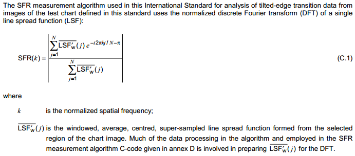
© ISO 2000 – All rights reserved
Here is the corresponding equation from ISO 12233:2014, Annex D. Note that E-SFR(k) is the symbol for edge-based SFR, not a subtraction:
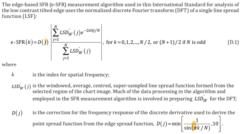
© ISO 2014 – All rights reserved
And here is the corresponding equation from ISO 12233:2017 Annex D.
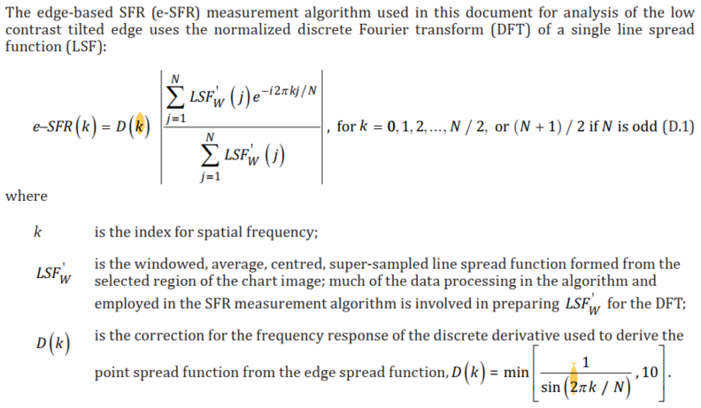
© ISO 2017 – All rights reserved
The difference between the 2014 and 2017 equations is the LSF (Line Spread Function) correction factor D(j) (D(k) in ISO 12233:2017), which corrects for the numerical differentiation used to calculate LSF (not the point spread function) from the Edge Spread Function. Note that D(j) (or D(k) ) are incorrect in both the 2014 and 2017 standards. They should read,
|
\(D(k) = minleft[frac{2pi k / N}{sinleft(2pi k / N right) },10right] = minleft[frac{1}{text{sinc}left( 2pi k / N right)},10 right] \)
|
*If you thought ISO standards were written by gods on
Mount Olympus, the many misprints should set you straight. |
Apart from min[…,10], this equation is used in ISO 12233:2022.
Show the equations for the numerical differentiation transfer functionHide the equations for the numerical differentiation transfer function
Numerical differentiation is a linear process with a transfer function
that differs from ideal differentiation.
The ISO 12233:2014 and 2017 formula (D.8) for calculating the Line Spread Function LSF(x) from the 4x-oversampled Edge Spread Function ESF(x) is,
\(displaystyle LSF_W(j) = W(j)frac{ESF(j+1) – ESF(j-1)}{2}\)
where W(j) is a windowing function not relevant to this analysis. Note that the difference spacing Δx in this calculation is 2 (4x-oversampled) samples = 0.5 pixels. This numerical difference formula may be rewritten,
\(displaystyle LSF(x) = frac{ESF(x + Delta x) – ESF(x – Delta x)}{2Delta x}\) where Δx = 1 pixel = 1 sample.
The Fourier transform (FT) for a time (or spatial) shift a is given in Wikipedia.
\(FT(g(x-a)) = e^{-iaomega} FT(g(x)) \)
For numerical differentiation where a = Δx, the Fourier transform is
\(displaystyle FT_{numerical} = frac{FT(g(x+a)-g(x-a))}{2a} = frac{e^{iaomega}-e^{-iaomega}}{2a}FT(g(x))\)
Noting that \(sin(x) = frac{e^{ix}-e^{-ix}}{2i}\) (see Wikipedia),
\(displaystyle FT_{numerical} = frac{sin(aomega)}{a}FT(g(x))\)
For pure differentiation, the Fourier transform is
\(displaystyle FT_{pure} = FTleft(frac{d g(x)}{dx}right) = omega FT(g(x))\)
The correction factor is therefore
\(displaystyle D(omega) = left|frac{FT_{pure}}{FT_{numerical}}right| = frac{aomega }{sin(aomega )}\)
Since Δx = a = 1 sample in 4x-oversampled space and ω = 2π f4x, where frequency f4x = ω/(2π) has units of cycles/sample in the 4x-oversampled space,
\(displaystyle aomega = 2pi f_{4x}\)
\(displaystyle D(f_{4x}) = left|frac{FT_{pure}}{FT_{numerical}}right| = frac{2pi f_{4x}}{sin(2pi f_{4x})} = frac{1}{text{sinc}(2pi f_{4x})}\) , where f4x is spatial frequency in cycles/(4x oversampled sample).
And since Δx = a = 1/4 pixel in (non-oversampled) pixel space,
\(displaystyle D(f_{CP}) = left|frac{FT_{pure}}{FT_{numerical}}right| = frac{pi f_{CP}/2}{sin(pi f_{CP}/2)} = frac{1}{text{sinc}(pi f_{CP}/2)}\) , where fCP is spatial frequency in cycles/pixel.
This is consistent with the statement in Annex K.4 that “the first zero of the filter response occurs at … 2 cycles/pixel. Equation (K.9) (the final equation for D) uses 2πk/N in place of πfCP/2 (or 2πf4x).
In Annex D, equation (D.10), D is expressed as
\(displaystyle D(k) = frac{2pi k/N}{sin(2pi k/N)} = frac{1}{text{sinc}(2 pi k/N)} \) , where k = 0, 1, 2, …, N/2 ((N+1)/2 if N is odd) is the index of spatial frequency.
where N is defined in Step (8) as “the length of the vector (4m).” Noting that 2πk/N = 2π f4x, i.e., f4x = k/N, the maximum spatial frequency is f4x = 1/2 (the Nyquist frequency in cycles/pixel).
2πk/N is used so D(k) can be substituted into equation (D.9), which is the equation for the discrete Fourier transform (DFT) for index k. In practice, a Fast Fourier Transform (FFT) is used to calculate MTF — it’s much faster than the DFT (N log2N instead of N2 operations).
Step (10)b says, “If the sampling interval is in units of pixels, then the spatial frequency values, f, will be expressed in units of cycles/pixel.”
This seems too us at Imatest to be a confusing and roundabout way to get frequency in cycles/pixel ( fCP).
It’s easiest to work directly in cycles/pixel, fCP, where the first null happens when fCP = 2 Cycles/pixel = 4×Nyquist frequency = 4 fNyq. It is significant that the x-axis in Figures K.1 and K.2 (MTF and e-SFR compensation for central-difference derivative operation) has units of Frequency in cycles/pixel — Imatest’s preferred units.
At the Nyquist frequency, fNyq = 0.5 Cycles/Pixel, \(D = frac{pi /4}{sin(pi /4)} = 1.1107\). At 2*Nyquist = 1 C/P, D = π/2 = 1.5708. To obtain D(k), substitute πk/N for aω/2. min[…, 10] keeps D(j) from becoming excessive where (πk/N ) >> sin(πk/N ).
|
Applying the correction factor
The LSF correction factor is enabled by default. To check or change the setting, click Settings (in the Imatest main window), Options III. You can check or uncheck the Use LSF… checkbox as appropriate, but we recommend leaving it checked. The checkbox sets derivCorr in the [imatest] section of imatest-v2.ini to 0 (correction off) or 1 (correction on).
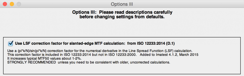 Options III window for applying or removing LSF correction factor
 Verification
To observe the effects of the LSF correction factor, we use an idealized edge, tilted 5 degrees, shown on the right. You can click on it to download it for your own testing.
The ideal edge increases uniformly from 0 to 1 over a distance of τ = 1 pixel.
|
The MTF of an ideal uniformly-increasing edge of width τ is the Fourier transform FT of its derivative, which is
\(displaystyle f(t) = frac{uleft((t+tau) / 2right) – uleft((t-tau) / 2right)}{tau}\) for unit step function u.
\(displaystyle FT(f) = frac{sin(pi tau f)}{pi tau f}\)
If τ is the sampling rate (the same as Δx or a in the green box, above),
\(displaystyletextrm{Nyquist frequency} = f_{textrm{Nyq}} = frac{1}{2tau}\)
The expected value of MTF at the Nyquist frequency (0.5 cycles/pixel) is
\(displaystyle FT(f_{textrm{Nyq}}) = frac{sin(pitau f_{textrm{Nyq}})}{pitau f_{textrm{Nyq}}} = frac{sin(pi /2)}{pi /2} = frac{2}{pi} = 0.6366\)
|
Here are the results without and with the LSF correction factor. Note that gamma has been set to 1 because the idealized image is not gamma-encoded. The results with LSF correction are much closer to the expected value of 2/π = 0.6366. The difference is likely due to digital sampling and the numerical binning/oversampling process: the average oversampled edge shown in the figures below is slightly rounded. Also, the edge rotation correction that is not applied to edges slanted by less than 8 degrees. The edge rotation is not included in the ISO standard and so is not applied to edges that fall under the ISO standard algorithm.
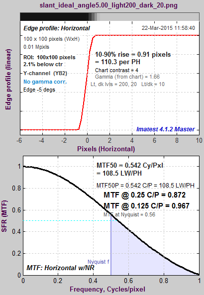 Ideal edge, uncorrected MTF. Ideal edge, uncorrected MTF.
MTF@Nyquist = 0.56. |
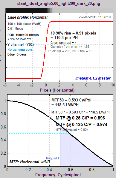 Ideal edge, LSF-corrected MTF. Ideal edge, LSF-corrected MTF.
MTF@Nyquist = 0.624. |
|
The figure on the right, generated by MTF Compare (a postprocessor to MTF calculation programs for comparing MTF calculations), compares the uncorrected MTF of the ideal edge (blue) with the corrected MTF (burgundy).
The black line is the uncorrected/corrected transfer function = 1/(correction factor D). It has the expected values of 0.9 (1/1.1107) at the Nyquist frequency (f = 0.5 C/P) and 2/π = 0.6366 at 2*Nyquist (1 C/P).
|
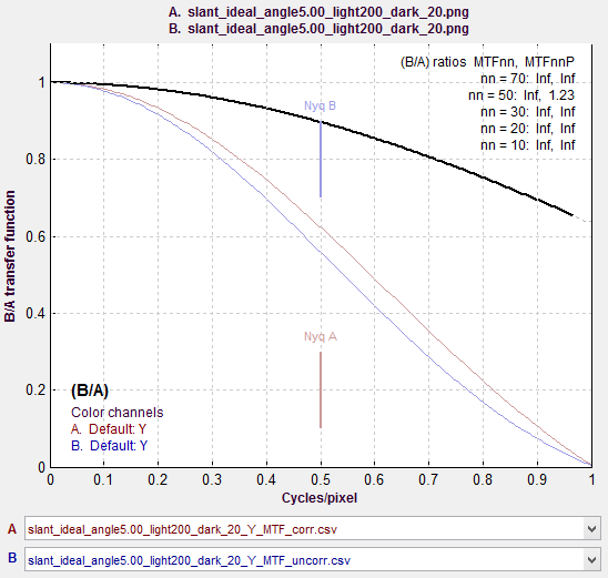 MTF Compare Uncorrected vs. Corrected MTF Compare Uncorrected vs. Corrected
|
Effects of gamma
Most color space files are gamma-encoded with gamma around 0.5, which is the default for Imatest slanted-edge SFR calculations. (Actual gamma varies considerably, and may be complicated by a tonal response curve on top of the gamma curve.) However, the ideal pulse is not gamma-encoded, so gamma = 1 is the appropriate setting. If gamma is set to 0.5 (the default), an inappropriate linearization will be applied to the edge, resulting in erroneous results: the MTF at 2*Nyquist is not equal to 0, as it should be.
|
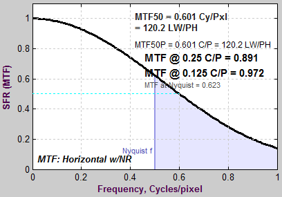 Ideal edge, uncorrected MTF, calculated Ideal edge, uncorrected MTF, calculated
(incorrectly) with gamma = 0.5 |
The idealized image has much more energy above the Nyquist frequency than typical high quality images. Here is an example for a high quality camera showing the effects of the LSF correction factor on MTF50— the most commonly-used summary metric.
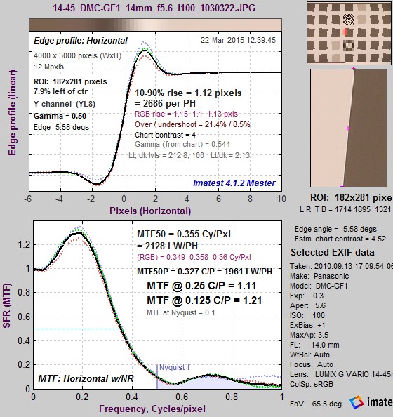 Typical edge, uncorrected MTF. Typical edge, uncorrected MTF.
MTF50 = 0.355 Cycles/Pixel. |
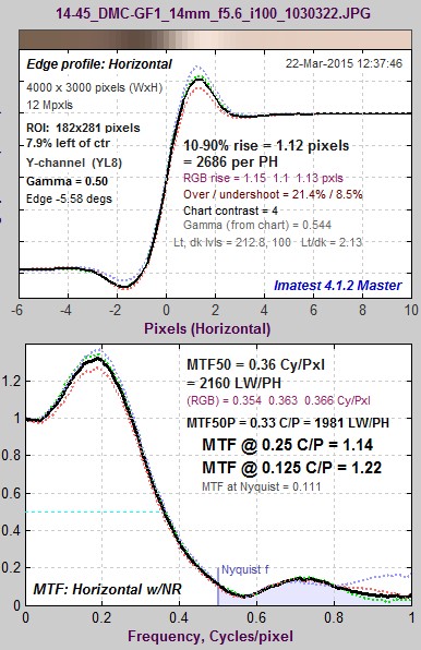 Typical edge, LSF-corrected MTF. Typical edge, LSF-corrected MTF.
MTF50 = 0.360 C/P: 1.41% higher. |
The difference may not be significant for many applications.
Consistency with older Imatest versions
The new correction factor is turned on by default in Imatest 4.2+ releases.
You can override the default, i.e., turn the correction factor on or off, by clicking Settings (in the Imatest main window), Options III, and checking or unchecking the Use LSF… checkbox as appropriate. Once the setting is saved, it will be retained across all future versions unless changed by the user. The default calculation be selected unless you manually change it in Options III window.
We strongly recommend leaving on the LSF correction factor, i.e., the box should be checked.
For industrial testing with pass/fail thresholds set up with the old calculation, we recommend either:
- adjusting your pass/fail specification to account for the measurement change
- continuing to use the old calculation by setting devCorr = 0 in the [imatest] section of the ini file
For example, on an ideal edge MTF at Nyquist/4 (0.125 C/P, a common KPI) is only increased by 0.64%, at Nyquist/2 (0.250 C/P) MTF is increased by 2.80%. On an actual sharp, RAW camera-phone image with Gamma=1, the MTF at Nyquist/4 is increased by 0.81%, MTF at Nyquist/4 is increased by 3.00%.


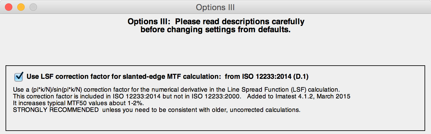 Options III window for applying or removing LSF correction factor