Published January 30 2015, updated July 26 2024
By Henry Koren, with contributions by Norman Koren.
Edited by Matthew Donato, Jackson Roland and Ty Cumby.

Table of Contents
View complete table of contents 3.4. Quality Staircase
2. Research and Development
2.1. Components
2.2. Imaging Lab
2.3. Configuration Files
2.3.1. Imatest INI File
2.3.2. Pass/Fail INI File
2.3.3. Edge ID File
2.3.4. Color Reference File
2.3.5. Tone Reference File
3. Manufacturing
3.1. Combining Tests
3.1.1. Light Field Test
3.1.2. Dark Field Test
3.1.3. Resolution Test
3.2. Guidelines
3.2.1. Data Collection
3.2.2. Early Intervention
3.2.3. Supplier Redundancy
3.3. Accuracy
3.3.1. Equipment and Environment
3.3.2. Test Target
3.3.3. Image Analysis
3.5. Measurement Challenges
3.5.1. Sharpness
3.5.1.1. Nonuniformity
3.5.1.2. Field Distance
3.5.1.3. Saturation
3.5.1.4. Target Quality
3.5.1.5. Space Utilization
3.5.2. Tilt and Rotation
3.5.2.1. Vertical Tilt
3.5.2.2. Convergence Angles
3.5.3. Blemish Detection
3.6. Equipment Verification
3.6.1. Sensor Baseline Noise
3.6.2. Optomechanics
3.6.3. Receptacle
3.6.4. Light source
3.6.4.1. Fluorescent
3.6.4.2. LED
3.7. Failure Analysis
4. Investigating External Quality
4.1. Sharpening
4.2. Noise Reduction
5. How to determine pass/fail criteria?
1. Introduction
The quality of imaging systems in mobile devices plays an increasingly important role in consumer purchasing decisions. A mobile device that fails to deliver acceptable quality images can have an adverse effect on the consumer’s brand loyalty, whether or not the customer has returned it.
Unless proper care is taken, raising camera quality standards can reduce manufacturing yield. This could damage a supplier’s profitability as well as endanger their ability to deliver the required production volume. The goal of this paper is to outline best practices for increasing quality standards so that both the producers and the consumers of the imaging system experience the best possible outcomes.
2. Research and Development
2.1. Components
The camera design team is responsible for selecting the camera components, which include the sensor, lens, housing, signal processing, as well as autofocus and optical image stabilization (OIS) mechanisms in many systems. The lens should be designed with sufficient sharpness to make good use of the sensor’s resolution (which can be very high in mobile devices).
The sensor’s pixel well size and quantum efficiency (QE) determine the fraction of incoming photon that affect the output digital value. The sensor’s anti-aliasing filter (if present) and color filter arrays also cause a reduction in the SFR (Spatial Frequency Response, i.e., sharpness) of the complete imaging system.
An understanding how individual components and interactions between components affect overall image quality is vital for developing performance specifications for testing imaging systems in manufacturing environments.
2.2. Imaging Lab
Imaging labs should be outfitted to provide an optimal environment for evaluating camera performance and image quality. The lab should include:
- A room where all ambient light can be blocked out.
- Reflective lighting that can evenly illuminate a test target without specular reflections.
- Targets that can fill the lens’s field of view at various test distances.
- Targets that have resolution that is significantly finer than the sensor under test.
- A target that has a tonal range that approaches or exceeds the dynamic range of the sensor under test. (The new ISO 15739 Dynamic Range calculation can estimate DR if the chart has a maximum density of base+2.)
- Light Meter.
- Sturdy tripod with clamp attachment.
- Dolly (which may include rail system) for changing the distance without tilting the DUT
Far more tests are typically done in the lab than in manufacturing. For example, Dynamic Range testing is extremely important in the development of imaging systems, but does not need to be tested in every camera. A simple noise or SNR (Signal-to-Noise Ratio) test should be sufficient.
The ideal test lab conditions may be difficult to reproduce in a manufacturing environment where space is limited. It is important to consider how limitations (most commonly, test chart resolution) will affect the quality metrics obtained in the manufacturing test.
2.3. Configuration Files
In addition to the physical configuration of the test environment, these test configuration files determine the parameters for the calculations performed by Imatest software.
2.3.1. Imatest INI File
The INI file contains settings which specify how a test image is to be decoded and analyzed and how results are to be displayed. Also contains properties of test environment; e.g., chart size and camera to chart distance which must be specified in order to produce accurate results. It also contains file names linking to related configuration files shown below.
2.3.2. Pass/Fail INI File
Defines specifications of acceptability, i.e., pass/fail thresholds. INI files are readable text files that can be edited in standard text editors. Imatest allows a great many pass/fail criteria to be selected. Completely new criteria have to be hard-coded (a relatively straightforward process). For more details, see the documentation page on Implementing Pass/Fail.
2.3.3. Edge ID File
Both Imatest SFRplus and eSFR ISO (ISO 12233:2014 target) have a large number of standard Region of Interest (ROI) selection options. But both allow an Edge ID file to be entered for cases where custom regions must be selected. The Edge ID file consists of one line per ROI, where each line has the format Nx_Ny_[LRTB]. Nx is the horizontal location of the square relative to the center (Nx = 0). Ny is similarly defined. [LRTB] represents either Left, Right, Top, or Bottom, respectively. Example: -1_2_R.
Edges should be selected to have a good mix of vertical and horizontal orientations in order to appropriately consider both sagittal and tangential directional MTF components. Region selection can be limited to a specific field distance (see section 3.5.1.2.). More details can be found in the SFRplus documentation.
2.3.4. Color Reference File
For color analysis, the default option is to use the standard values, which are derived from the X-Rite Colorchecker, but which may not closely match the values of the actual printed chart. If greater precision is required, values for different reflective media types (matte and semigloss) can be selected.
For the most precise analysis you can enter a custom reference file containing L*a*b* data for color patches. Some charts are supplied with reference files. Color reference files are produced using a spectrophotometer, which saves measurements in CGATS or CSV format.
2.3.5. Tone Reference File
For tone analysis you the default option is to use the standard values which are 0.1 density steps. This may not exactly match the density values of the actual printed chart. If greater tonal response measurement precision is required, you can enter a custom reference file containing density data for the grayscale patches. Some charts, such as the Imatest 36-patch Dynamic Range chart, are supplied with reference files. Tonal reference files can be produced using a densitometer or spectrophotometer, and the file is formatted either in CGATS, or CSV format where one density value is listed on each line, low to high density.
3. Manufacturing
Because of the implications of poor quality imaging systems, it is of critical importance that each and every device that is produced goes through a rigorous image quality testing procedure.
3.1. Combining Tests
Imatest’s test charts and software allow many image quality factors to be measured using a single image. For a complete manufacturing test, as few as three images may be required.
3.1.1. Light Field Test
Also known as the Blemish test, this involves analyzing an image of a uniform light source for:
- Optical Center (OC)
- Visible blemishes on sensor (dust, spots)
- Defect Pixels (DP) – hot/dead with absolute thresholds or light/dark with relative thresholds. Including cluster detection.
- Color Uniformity (CU)
- Relative Illumination (RI)
- Color/illumination calibration data written to sensor with one-time programming (OTP)
3.1.2. Dark Field Test
Blocking all light from entering the lens and the dark image is analyzed for:
- Dark Noise (defect pixels with an absolute threshold)
- Dark Uniformity
- Hot Spots (light blemishes)
3.1.3. Resolution Test
Imatest’s flagship SFRplus and eSFR ISO test targets can be used to measure a great many image quality factors with a single image, including:
- Resolution (MTF or SFR) mapped over the image surface. For manufacturing tests, resolution in center and corners are often selected.
- Lens-to-sensor tilt (outer MTF imbalance)
- Sensor-to-chart tilt and offset.
- Rotation, Distortion, Field of View.
- Bayer filter position verification.
- Image orientation verification.
- Autofocus voice coil motor (VCM) calibration.
eSFR ISO charts have somewhat less spatial detail than SFRplus charts, but offer more detailed noise and Dynamic Range measurements.
In order to test across a range of distances, near and far, it may be necessary to repeat this test using more than one chart.
3.2. Guidelines
In order to achieve the best possible outcome we recommend a quality management protocol that embraces the following principles.
3.2.1. Data Collection
Throughout the manufacturing process, images and test results should be collected by the overseers of project quality
- Images – should be collected so that measurements can be independently reproduced. Ideally they should be raw images, which are unaffected by signal processing, and hence more likely to produce consistent measurements.
- JSON test result data – The output file produced by running a test on a particular image, including pass-fail results and full test results.
Comprehensive data collection enables:
- verification that test standards were adhered to throughout the supply chain,
- detection of tampering with the spec or configuration files,
- traceability so that the root causes of failures can be identified.
3.2.2. Early Intervention
For all phases of manufacturing it is best to catch problems before the component or device is completed. The earlier a problem is caught, the fewer the negative consequences:
- Lens and sensor makers should control for the quality of the materials they use to build their components (this does not involve Imatest).
- Module makers should optically test the individual lens components and assembled lenses to ensure that lens quality meets the design goals.
- Module makers should verify sensor quality before attaching the assembled lens.
- Device manufacturers should verify module quality before assembling the device.
Problems which aren’t caught earlier, should be caught later:
- Device manufacturers should verify device quality at the end of the line.
- Device buyers should verify the quality of the manufactured device.
- Reverse logistics should verify the quality of a returned device.
3.2.3. Supplier Redundancy
For large scale device manufacturing it is advisable to have multiple camera module manufacturers so that one supplier’s quality or logistics issues do not adversely affect the entire project. If one supplier fails to produce the required quality, another should be prepared to step up.
3.3. Accuracy
In order to reproduce results from different types of test equipment at different companies and locations, it is important to quantify as many factors which affect image as possible.
Differences or deficiencies in any of the below measurement system properties could potentially increase variability of results or cause systematic errors.
3.3.1. Equipment and Environment
- Distance(s) between the camera and the target(s) – multiple for autofocus tests.
- Method of securing the unit under test within the fixture.
- Aligning the central axis of the unit under test to the center of the test target.
- Light source:
- Radiance and spectral properties.
- Spatial uniformity.
- Temporal consistency (flicker-free).
- Presence of ambient or external light sources.
- Elements in the light path:
- Glass sheets to hold the chart.
- Conversion optics for simulating a longer test distance.
- Motion generation for optical image stabilization (OIS) tests:
- Amplitude and frequency of motion.
- Direction of motion (motion profile).
- Synchronization of capture initiation with motion profile.
- Sensor settings:
- Exposure time.
- ISO speed (analog gain).
- Other registry settings – defect pixel correction, mirror/flip, etc.
- Hardware interface for image acquisition.
- Processing performed on image prior to analysis (ideally none).
3.3.2. Test Target
- Analysis feature types – slanted edges, stars, wedges, multiburst patterns, etc.
- Feature locations – % distance from center to corner. (relative to target distance)
- Contrast ratio for spatial analysis.
- Density level for tonal analysis.
- Production process precision.
3.3.3. Image Analysis
- For color sensors, the method of determining the color channels (demosaicing).
- The selection of test regions of interest (ROIs) for analysis:
- Location within the field.
- Size (For slanted edge-SFR, larger regions are more stable).
- Orientation (horizontal, vertical, or other angles).
- Gamma linearization settings (none for raw sensor data).
- Algorithm for producing detailed outputs.
- Selected quality indicators extracted from outputs.
3.4. Quality Staircase
Even if all potential sources of variation are minimized there will remain some amount of variation due to the noise that is inherent in a sampled imaging system. This means that some units whose quality metrics could fall close to the threshold of acceptability may alternate between passing and failing results if tested repeatedly.
In order to prevent this kind of variation from resulting in failures further down the line, higher standards for quality should be set for the earlier component and module tests than the standards which are set for the final assembly test.
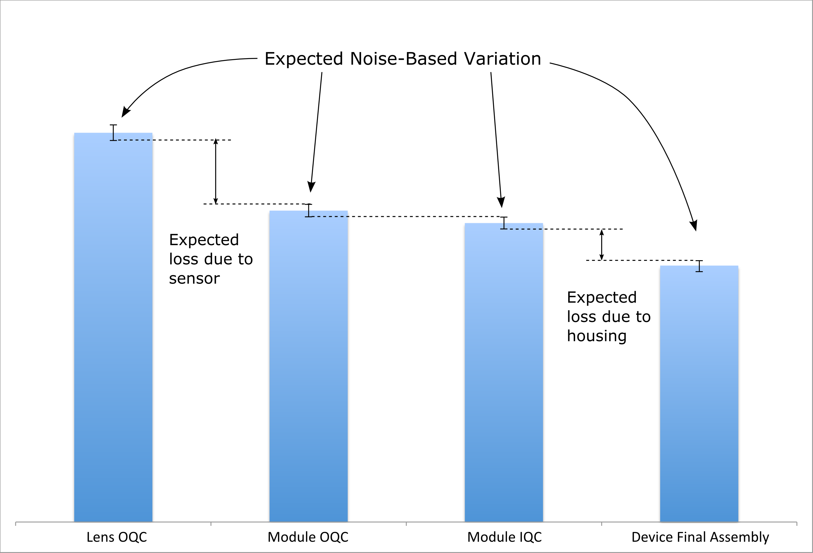
This principle is also important since the module installed in the device often passes through an additional layer of glass enclosure that would lead to some reduction in quality compared to the naked camera module.
3.5. Measurement Challenges
3.5.1. Sharpness
Verifying the camera’s ability to achieve focus across the image plane is a critical requirement for manufacturing tests. Purely optical problems with the lens, including astigmatism, coma, lateral and axial and spherical aberration can be identified with optical lens testing systems, while image sharpness problems such as defocus, lens tilt, autofocus mechanism (VCM) failure and optical image stabilization (OIS) failure can be assessed using an image system test of the type provided by Imatest.
3.5.1.1. Nonuniformity
The mean MTF taken over the entire image plane is insufficient to determine whether a lens should pass or fail. More detail is required. For example, a tilted lens whose peak sharpness is shifted away from the center of the sensor might have lower MTF values on one side of the image, but could have higher MTF on the other. The average MTF of the outer corner regions will not detect when a single corner of the image has fallen below spec.
Imatest performs a number of measurements that can address sharpness nonuniformity. In one method, SFRplus divides the outer areas of the image up into four quadrants, then computes means of all the slanted-edge regions within each quadrant. A Pass/fail parameter outer_quadrant_mean_min_min defines the minimum allowable MTF value for the least sharp corner of the image.
3.5.1.2. Field Distance
The selection of the regions to be tested within the image may be tailored in order to closely match up with the MTF specifications provided by the lens manufacturer, which define expected MTF values as a function of the field distance: zero for the geometric center of the lens, one for the corner.
A particular field distance (typically between 0.7 and 0.8) can be targeted for analysis of the sharpness of the outer areas of the image. Since the test regions may not be available at exact positions, a set of regions with a mean field distance that is close to the targeted field distance can be analyzed.

0_0_T
0_0_B
0_0_L
0_0_R
-3_-2_L
-4_-2_B
-3_2_L
-4_2_T
-4_-1_B
-4_-1_R
-4_1_R
-4_1_T
3_-2_R
4_-2_B
3_2_R
4_2_T
4_-1_B
4_-1_L
4_1_L
4_1_T
Here an example selection of 20 regions which average out close to a 0.75 (75%) field distance, covers all four corners, and has an equal number of vertical and horizontal test regions.
The edges to be tested are defined in the Edge ID File (see section 2.3.3.). For more details see our article: Selecting SFR edge regions based on field distance
3.5.1.3. Saturation
If portions of an image reach the maximum allowable pixel level (255 for most 24-bit color files; 2n-1 for sensors with bit depth = n) or the minimum allowable level (0), the image is saturated. Saturation adversely affects most image quality measurements, but it can be particularly damaging for slanted-edge MTF measurements if there are sharp corners at the saturation boundaries. These corners contain high-frequency energy that artificially boosts MTF measurements.
Saturation was a frequent problem in images of the old ISO 12233:2000 test chart, which is specified as having a minimum contrast of 40:1. It is less of a problem with older SFRplus charts, which have 10:1 contrast, and it’s rarely a problem with newer 4:1 contrast SFRplus and ISO 12233:2014 charts. But we have seen highly overexposed images of 4:1 charts that were seriously saturated, and hence had higher MTF than if they were properly exposed. This may have been done intentionally to pass camera modules that would have otherwise failed.
Improperly exposed images due to incorrect exposure time, sensor gain, or chart illumination level can cause saturation. For this reason, several measurements related to saturation are included in the pass/fail criteria, including the mean pixel level near the center of the image, the fraction of the image above 99% of the saturation level, and the fraction below 2% of the saturation level. In general, saturation should be interpreted as a failure of the test setup rather than a failure of the UUT. See this article for more details about saturation.
3.5.1.4. Target Quality
In the development lab, the test target (scaled to the image sensor size) should ideally be much sharper than the sensor can resolve. This requirement, along with sensor resolution, angular field of view, and range of allowable focus distances, affects the choice of chart size and media.
Imatest SFRplus and eSFR ISO charts are available in a hierarchy of sizes and precisions: inkjet (largest but lowest precision), photographic paper (many charts under development), Black and White photographic film, Color photographic file, and (smallest and highest precision) chrome-on-glass. We have investigated the quality of both transmissive as well as reflective substrate types.
In manufacturing environments, space constraints may force compromises in the selection of charts: they may need to be smaller than optimum, and MTF measurements may be reduced as a result. This is acceptable as long as there is a clear understanding of the compromise and pass/fail thresholds are appropriately adjusted.
See our documentation on chart quality for more details. The Imatest Chart Finder can be helpful for chart selection.
3.5.1.5. Space Utilization
For modules designed to focus at longer distances, performing resolution tests that approach that distance within a limited footprint on the factory floor is a difficult challenge.
Collimating optics, which may include relay (or conversion) lenses or mirrors, enable the creation of a virtual image that appears to be at a different distance. This typically increases the virtual distance of high precision test targets, but could also be reversed so that large targets appear closer.
Collimators degrade the quality of the test target image to some degree. An ideal collimator would have:
- A virtual image that is at or beyond the maximum hyperfocal distance.
- Testable regions that will not impact the measured MTF.
- Testable regions that are on the outside of imaging plane (off-axis)
Unfortunately, a single collimator, or combination of collimators with these properties would almost certainly be cost-prohibitive, so compromises must be made:
- A virtual image that is within the maximum hyperfocal distance.
- Testable regions that will have some adverse effect on the measured MTF which should be compensated for by adjusting the pass/fail spec.
- Testable regions that will not extend to the outer field, potentially only in the center
- Motion control systems can be used to shift the collimator off axis (slower)
- Motion control systems can rotate around the outside of the outer field (slower).
3.5.2. Tilt and Rotation
3.5.2.1. Vertical Tilt
The SFRplus detection algorithm requires that the image contains some white space above the top horizontal bar and below the bottom horizontal bar. (It is OK for the sides of the bar extend beyond the image.) For this reason, the maximum allowable vertical tilt angle (θVtiltmax) must be limited so there is always some space outside the horizontal bars. In other words, the bars should be contained entirely within the Vertical Field of View (VFoV).
The distance between the top of the top bar and the bottom of the bottom bar in the SFRplus chart is called the “bar-to-bar height”, (hbars). dtest is the camera-to-chart distance. In order to determine the maximum bar to bar height (hbars ) of the chart, the following equations can be used:

Based on the total image plane height of:

3.5.2.2. Convergence Angles
The vertical and horizontal convergence angles define the amount of keystone (or perspective) distortion in the chart image. They are not the same as the physical tilt angles of the device.
In SFRplus the Horizontal Convergence Angle (HCA) is determined by extending the SFRplus distortion bars until they meet. The angle is normalized to lines that intersect the top and bottom centers of the image.

The Vertical Convergence Angle (VCA) is determined from a column of square edges near the left and right image boundaries. Like the HCA, it is normalized for lines that intersect the left and right image boundaries.
In eSFR ISO the HCA and VCA are determined from the registration marks, using a similar normalization to the image edges.
Meaning of the convergence angle signs:
| Convergence Angle | + Positive | – Negative |
| Vertical (VCA) | converges to top | converges to bottom |
| Horizontal (HCA) | converges to left | converges to right |
For more details about tilt, see our article “Measuring the effects of tilt”.
3.5.3. Blemish Detection
To identify units that should be rejected due to blemishes on the sensor, the typical use cases of the images— image size and viewing distance – must be considered.
Imatest’s Blemish Detect module contains a pair of spatial filters that can be tuned to approximate the human visual system’s contrast sensitivity function, which is a bandpass filter with peak response around 4 cycles/degree. The highpass filter removes low-frequency nonuniformity (light falloff / lens shading / vignetting). The lowpass filter removes high-frequency noise. Together these filters can be tuned to emulate the human visual system for a range of viewing conditions.
While many blemishes are clearly distinguishable by both man and machine, many with low contrast and/or spatial frequency content far from the human visual system’s peak response (i.e., too large or small) may not be visible. These include oily smudges and dust particles that may be separated from the active sensor surface by as much as 1 mm (micro-lenses and bayer, IR, and anti-aliasing filters). The goal of tuning the blemish detection parameters is to distinguish perceptible from imperceptible blemishes. The following process is recommended:
- Collect a large set of even light field images from a set of built devices, making sure to include a significant number that contain varying sizes of blemishes. If the source of real imagery is limited, it can be useful to add simulated blemishes above and below the threshold of perceptibility to some images.
- Using a controlled viewing environment where image size and viewing distance are fixed, have a human inspect these images for blemishes, separating them into Pass & Fail groups.
- Using the latest settings, run the Imatest Blemish Detect routine on the same batch of images
- Identify false positives: where blemishes that are not perceptible to the human viewer are flagged
- Identify false negatives: where blemishes that were perceptible to the human viewer are not flagged
- For each false result, attempt to tune the Blemish Detect filter and threshold settings in order to rectify the problem.
- Repeat step 3-7 until the false results are minimized or eliminated.
A large sample of test images containing a variety of blemishes above and below the threshold of perceptibility will enhance confidence in the validity of the settings. After this optimization process is completed, the algorithms will run independently without any human involvement.
For more details, see our Blemish detect documentation.
3.6. Equipment Verification
In order to verify that a camera test machine is performing nominally, engineers should perform Gage Range and Repeatability (GR&R) test. This both validates the image processing measurement system, and also a verifies the complete system performance stability, including the repeatability of the fixture between removal and replacement of the module, the stability of the light source in the fixture, and the ability of the sensor and signal processing to produce consistent outputs within a specific test region.
There are two important aspects of a Gauge R&R: [source: wikipedia]
- Repeatability: The variation in measurements taken by a single person or instrument on the same or replicate item and under the same conditions.
- Reproducibility: the variation induced when different operators, instruments, or laboratories measure the same or replicate specimen.
An example of GR&R plan:
- 8 modules/devices that have a range of quality levels: including good, bad, and borderline units.
- 3 different operators (not applicable for fully-automated test machines)
- 4 different repetitions of the test
As the above numbers are increased the confidence in the GR&R test will also increase. Minitab statistical analysis software or other means of calculating can be used to process the test equipment output data and produce the GR&R report.
If the Gage R&R test fails, the next step is to identify the primary contributors to variation so they can be minimized.
3.6.1. Sensor Baseline Noise
Noise is the main source of variability in compact cameras, especially as pixel size decreases. Noise based variation can be understood by capturing and analyzing a sequence of images from the same module without any changes between each capture. We will call this the “baseline noise variation”.
Steps can be taken to reduce the amount of noise:
- Keeping the light level bright enough (but not too bright) will allow for capture of low-noise images using low ISO speeds.
- Signal averaging may be used to reduce the noise by combining multiple images (can slow down the test speed)
And steps can be taken in order to reduce the effect of the noise:
- In the even field tests, low pass filters remove noise before blemish detection
- In the slanted-edge SFR resolution test: increasing the size and the number of test regions
- In the slanted-edge SFR resolution test: using Imatest’s MTF noise reduction feature (modified apodization).
3.6.2. Optomechanics
The Voice Coil Motor (VCM) mechanism is perhaps the greatest potential contributor to variation in autofocus (AF) module tests. The hysteresis of the motor systems can mean that a slightly different focus position is reached depending on the history of the recent positions focused at before.
In order to understand the effect of AF on repeatedly capturing images, a couple different experiments are called for. The results of these experiments should be compared to the baseline noise variation.
The hysteresis of the AF system can be understood by moving the focus position away from and then back to the selected focus position between captures. You can understand the stabilization properties of the AF by first moving away from a focus position, then capturing the image for analysis after commanding the AF to go to the same selected focus position several times.
3.6.3. Receptacle
When the device or module is inserted into the testing fixture, a mechanical system should produce precisely repeatable positioning. Any translation or rotation due to the receptacle will be difficult to distinguish from actual problems with the UUT.
An experiment where the module is removed from, then re-inserted into the fixture between repeated tests (also known as “pick and place”) will allow you to determine the variation caused by the fixture.
Metrics to compare to the baseline noise variation include:
- Offset between center of the light source or test target and the center of the image.
- Horizontal and vertical convergence angles (sensor to target tilt)
- Rotation
- Field of view (distance variation)
3.6.4. Light source
Flickery light sources are common sources of GR&R failure for sensors with rolling shutter where each row of pixels within image comes from a different window of time. Any flicker in the light source will manifest itself as horizontal banding when the period of light intensity change is any longer than the integration time of a row of pixels.
Output metrics to compare to the baseline noise variation:
- Relative Illumination (RI)
- Color uniformity (CU)
Since the banding must overlap with a measurement patch in order to affect the pass/fail outputs, inspecting Imatest’s vertical uniformity profile, or inspecting Imatest’s detailed uniformity contour plots can allow the banding to be identified from a single image. Otherwise, a large enough set of images should be analyzed so that one of the bands is likely to have coincided with the location of the measurement patches.
3.6.4.1. Fluorescent
For fluorescent light sources, high frequency ballasts (on the order of 60 kHz) are used to prevent flicker from manifesting itself as banding. Ballast frequency alone does not guarantee light source stability. The design quality of the ballast can influence the light sources ability to withstand power source noise issues that may arise from nearby loads (particularly electric motors) that are not sufficiently isolated. Noise filtering surge protectors can be utilized to mitigate power supply related instability.
Fluorescent lights will also dim and could begin to have issues with flickering as they aproach their end of life, this should be detectable using Imatest SFRplus’ Chart_mean_pixel_level_bounds pass/fail parameter.
3.6.4.2. LED
For LED light sources, Pulse width modulation (PWM) as a method for limiting LED brightness can introduce flicker. Constant current reduction (CCR) is a preferable method for attenuating LED luminance.
3.7. Failure Analysis
When a camera fails at any stage of manufacturing, or later fails out in the field, the detailed test data that was collected on that camera may become useful to preventing a recurrence of the failure.
Although many potential metrics that can be produced by Imatest’s SFRplus chart and analysis algorithms may not immediately be utilized for passing or failing units, these detailed features are very useful for performing postmortem analysis. Images of simplified test charts such as ones that only have limited resolution analysis features in the centers and corners are fairly useless for performing appropriate detailed failure analysis.
If a device gets returned by a customer, it should be tested again as part of the reverse logistics program. A determination should be made if the imager has malfunctioned or fallen below spec while out in the field. Tracing the detailed history of the test results earlier in the modules lifetime could potentially reveal clues about how a spec adjustment or test program modification could enable catching a similar failure earlier.
4. Investigating External Quality
Signal processing is often used to mitigate the deficiencies of low-quality optics and optoelectronics. To verify the quality of a camera module’s physical components, it is best to analyze raw or minimally-processed image sensor output.
This may be difficult to accomplish in practice. If raw or minimally-processed images are unavailable, the effects of the camera’s signal processing will need to be understood in order to properly judge the total camera system performance.
4.1. Sharpening
Sharpening is a signal processing step that improves perceptual sharpness and MTF measurements by boosting high spatial frequencies. Most consumer cameras have non-uniform signal processing where the strongest image sharpening takes place near contrasty features like edges.
All digital images – without exception – benefit from sharpening, but image quality is frequently degraded by excessive sharpening, which can cause highly visible “halos” near edges. Image quality is also compromised if there is insufficient sharpening. Imatest can measure the amount of sharpening and determine whether it is within the optimal range, which depends on the application
Sharpening is best measured with slanted-edges in the recommended SFRplus or eSFR ISO modules. It can be measured in two domains. In the spatial domain it is quantified as overshoot and undershoot. Overshoot greater than 25% may be objectionable, depending on the application. In frequency domain we define “oversharpening” as 100% – MTF at 0.15 cycles/pixel (0.3 * Nyquist). In our experience OS = 0 corresponds to a conservatively sharpened image with a slight (barely visible) overshoot. Oversharpening over 25% may be objectionable while oversharpening less than 0 indicates that the image may benefit from more sharpening.
If cameras are tested using sharpened images, it is important to know the degree of sharpening, and it is critical that the sharpening be consistent for all tests. See the Imatest documentation page on sharpening for more details.
4.2. Noise Reduction
Noise can cause a significant degradation in perceptual image quality. It can be especially serious in cameras with small pixel size – such as you find in most mobile devices.
Typically, noise reduction involves the attenuation of high spatial frequencies (lowpass filtering), which reduces MTF. It is largest in the absence of contrasty features, i.e., it tends to be maximum where sharpening is minimum. Noise reduction can cause a loss of low-contrast high spatial frequency detail – fine texture.
Imatest can measure the loss of detail caused by noise reduction with several test charts and modules.
Noise and Dynamic range (which is closely-related) can be measured by grayscale patterns using Color/Tone Interactive, Color/Tone Auto, or eSFR ISO. Depending on the application, we recommend the 36-patch transmissive Dynamic Range chart, the ISO 14524 or ISO 15739 charts, or the 20-patch grayscale pattern that is automatically analyzed by eSFR ISO.
The loss in detail due to noise reduction can be examined using the Log F-Contrast chart and module.
The Spilled Coins chart and module (Imatest’s version of Dead Leaves) represents a typical image with low contrast features. Its MTF can be compared with the slanted-edge as an indication of loss of detail.
Although the loss of fine detail due to noise reduction is important to understand during imaging system development, it tends to be less important for manufacturing testing because it has relatively little effect on the slanted-edge sharpness measurements.
5. How to determine pass/fail criteria?
Deciding on pass-fail criteria is challenging and involves multiple tradeoffs between system performance, component cost, and manufacturing yield.
Ideally, in the research and development phase of designing your camera system, a lens, sensor, signal processing, and camera body components will be selected that will adequately perform the human and/or machine vision task you need to have performed.
- For human vision, you may consider a collection of perceptually related Image Quality factors such as those included in ISO CPIQ or VCX standards.
- For machine vision, you may consider image quality factors where if your system does not provide sufficient quality, the computer vision task will fail. Beyond traditional image quality factors consider information metrics as a quality factor that will include sharpness and noise in a single measurement.
Once you have decided on the components that will comprise your imaging system, you should build and test a collection of sample cameras. Depending on the precision of you and your suppliers’ manufacturing and assembly processes, these samples will fall within a distribution of quality.
In manufacturing, a golden sample is a perfectly made component. If you use a single golden sample to set your pass-fail criteria, you would want to repeat several tests with that sample in order to determine its minimum quality in the presence of sources of variation because of sensor noise and other factors. You also should consider where in the production line you are doing the testing and how the Quality Staircase impacts quality loss.
But if you only consider a single “golden sample”, you may find that other cameras that are not quite as good as the golden sample but “good enough” will fail. So we introduce the term “bronze sample” to represent a device that barely meets your needs, but if it was any worse in quality, it should fail. You should select a bronze sample based on your application needs (see above). Then you should select pass fail criteria just below what your bronze sample is able to achieve so that your bronze sample will always pass.
As you ramp to mass production, you should consider the production yield. If the pass-fail threshold threshold you select leads to a production yield that is too low:
- you may need to reconsider your selection of components in order to get improved quality (return to R&D).
- you may need to increase the requirement for quality from your suppliers and your incoming quality control step.
- you may need to improve your internal manufacturing tolerancing when it comes to the final assembly of your camera’s subassemblies.
If you need additional help navigating this process, Imatest consulting services could help you to make better-informed decisions about your camera quality.
See also Understanding collimator MTF loss using bronze and golden sample testing.